

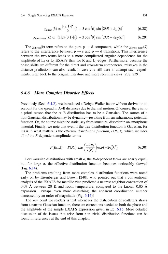
χ direct k
ð Þ /
2j1
h i
j
j
2
2
1 þ 3 cos
2
θ
À
Á
sin 2kR þ δ 2j k
ð Þ
Â
Ã
ð6:28Þ
χ cross‐term k
ð Þ / 1j2
h ih0j1i
j
j1 À 3 cos
2
θ
À
Á
sin 2kR þ δ 02j k
ð Þ
Â
Ã
ð6:29Þ
The χ direct (k) term refers to the pure p ! d component, while the χ cross-term (k)
refers to the interference between p ! s and p ! d transitions. This interference
between the two terms leads to a more complicated angular dependence for the
amplitude of L 3 or L 2 EXAFS than for K and L 1 -edges. Furthermore, because the
phase shifts are different for the direct and cross-term components, mistakes in the
distance predictions can also result. In case you still dare to attempt such experiments, refer back to the original literature and more recent reviews [238, 239].
6.4.6 More Complex Disorder Effects
Previously (Sect. 6.4.2), we introduced a Debye-Waller factor without derivation to
account for the spread in A–B distances due to thermal motion. Of course, there is no
a priori reason that the A–B distribution has to be a Gaussian. The source of a
non-Gaussian distribution may be dynamic—resulting from an anharmonic potential
function. Or, the source might be static, say from structural disorder in an amorphous
material. Finally, we note that even if the true distribution function is Gaussian, for
EXAFS what matters is the effective distribution function, P(R b ,λ), which includes
all of the R-dependent amplitude terms:
P R b , λ
ð
Þ¼P R b
ð Þ exp
À2R b
λ k
ð Þ
exp À2σ
2
b k
2
À
Á
ð6:30Þ
For Gaussian distributions with small σ, the R-dependent terms are nearly equal,
but for large σ, the effective distribution function becomes noticeably skewed
(Fig. 6.14).
The problems resulting from more complex distribution functions were noted
early on by Eisenberger and Brown [240], who pointed out that a conventional
analysis of the EXAFS for metallic zinc predicted a nearest neighbor contraction of
0.09 Å between 20 K and room temperature, compared to the known 0.05 Å
expansion. Perhaps even more disturbing, the apparent coordination number
decreased by an order of magnitude (Fig. 6.14)!
The key point for readers is that whenever the distribution of scatterers strays
from a narrow Gaussian function, there are corrections needed to both the phase and
the amplitude of the simple EXAFS expression given in Eq. 6.15. More detailed
discussion of the issues that arise from non-trivial distribution functions can be
found in references at the end of this chapter.
6.4 Single Scattering EXAFS Equation
151
ð Þ /
2j1
h i
j
j
2
2
1 þ 3 cos
2
θ
À
Á
sin 2kR þ δ 2j k
ð Þ
Â
Ã
ð6:28Þ
χ cross‐term k
ð Þ / 1j2
h ih0j1i
j
j1 À 3 cos
2
θ
À
Á
sin 2kR þ δ 02j k
ð Þ
Â
Ã
ð6:29Þ
The χ direct (k) term refers to the pure p ! d component, while the χ cross-term (k)
refers to the interference between p ! s and p ! d transitions. This interference
between the two terms leads to a more complicated angular dependence for the
amplitude of L 3 or L 2 EXAFS than for K and L 1 -edges. Furthermore, because the
phase shifts are different for the direct and cross-term components, mistakes in the
distance predictions can also result. In case you still dare to attempt such experiments, refer back to the original literature and more recent reviews [238, 239].
6.4.6 More Complex Disorder Effects
Previously (Sect. 6.4.2), we introduced a Debye-Waller factor without derivation to
account for the spread in A–B distances due to thermal motion. Of course, there is no
a priori reason that the A–B distribution has to be a Gaussian. The source of a
non-Gaussian distribution may be dynamic—resulting from an anharmonic potential
function. Or, the source might be static, say from structural disorder in an amorphous
material. Finally, we note that even if the true distribution function is Gaussian, for
EXAFS what matters is the effective distribution function, P(R b ,λ), which includes
all of the R-dependent amplitude terms:
P R b , λ
ð
Þ¼P R b
ð Þ exp
À2R b
λ k
ð Þ
exp À2σ
2
b k
2
À
Á
ð6:30Þ
For Gaussian distributions with small σ, the R-dependent terms are nearly equal,
but for large σ, the effective distribution function becomes noticeably skewed
(Fig. 6.14).
The problems resulting from more complex distribution functions were noted
early on by Eisenberger and Brown [240], who pointed out that a conventional
analysis of the EXAFS for metallic zinc predicted a nearest neighbor contraction of
0.09 Å between 20 K and room temperature, compared to the known 0.05 Å
expansion. Perhaps even more disturbing, the apparent coordination number
decreased by an order of magnitude (Fig. 6.14)!
The key point for readers is that whenever the distribution of scatterers strays
from a narrow Gaussian function, there are corrections needed to both the phase and
the amplitude of the simple EXAFS expression given in Eq. 6.15. More detailed
discussion of the issues that arise from non-trivial distribution functions can be
found in references at the end of this chapter.
6.4 Single Scattering EXAFS Equation
151