

6.4.2 Simple Disorder Effects: Debye-Waller Factors
In a real sample, the distances between absorber and backscatterers are not fixed.
Instead, there is always a distribution of distances, because of both thermal motion
(dynamic disorder) and structural (static) disorder. We can describe this distribution
of distances in terms of a pair distribution function P(r)dr that defines the probability
that the absorber-backscatterer distance lies between r and r + dr. The distribution of
distances around the centroid R AB means that the observed EXAFS signal will be a
sum of sine waves with different frequencies, and the interference between these
frequencies will modify the amplitude and (sometimes) phase of the EXAFS.
6.4.2.1 Diatomic Systems
As the simplest case, consider a bimolecular system A–B, with masses m A and m B
and force constant k A-B . Although in the classical limit the two masses could sit at a
fixed distance R A-B , we know from quantum mechanics that this harmonic oscillator
will have a “zero-point motion” even at a temperature of absolute zero.
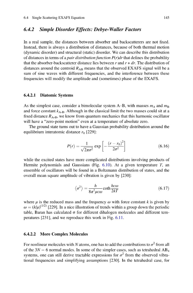
The ground state turns out to have a Gaussian probability distribution around the
equilibrium interatomic distance r 0 [229]:
P r
ð Þ ¼
1
ffiffiffiffiffiffiffiffiffi ffi
2πσ 2
p
exp À
r À r 0
ð
Þ
2
2σ 2
!
ð6:16Þ
while the excited states have more complicated distributions involving products of
Hermite polynomials and Gaussians (Fig. 6.10). At a given temperature T, an
ensemble of oscillators will be found in a Boltzmann distribution of states, and the
overall mean square amplitude of vibration is given by [230]:
σ
2
¼
h
8π
2
μcω
coth
hcω
2kT
ð6:17Þ
where μ is the reduced mass and the frequency ω with force constant k is given by
ω ¼ (k/μ)
(1/2) [229]. In a nice illustration of trends within a group down the periodic
table, Baran has calculated σ for different dihalogen molecules and different temperatures [231], and we reproduce this work in Fig. 6.11.
6.4.2.2 More Complex Molecules
For nonlinear molecules with N atoms, one has to add the contributions to σ
2 from all
of the 3N À 6 normal modes. In some of the simpler cases, such as tetrahedral AB 4
systems, one can still derive tractable expressions for σ
2 from the observed vibrational frequencies and simplifying assumptions [230]. In the tetrahedral case, for
6.4 Single Scattering EXAFS Equation
145
In a real sample, the distances between absorber and backscatterers are not fixed.
Instead, there is always a distribution of distances, because of both thermal motion
(dynamic disorder) and structural (static) disorder. We can describe this distribution
of distances in terms of a pair distribution function P(r)dr that defines the probability
that the absorber-backscatterer distance lies between r and r + dr. The distribution of
distances around the centroid R AB means that the observed EXAFS signal will be a
sum of sine waves with different frequencies, and the interference between these
frequencies will modify the amplitude and (sometimes) phase of the EXAFS.
6.4.2.1 Diatomic Systems
As the simplest case, consider a bimolecular system A–B, with masses m A and m B
and force constant k A-B . Although in the classical limit the two masses could sit at a
fixed distance R A-B , we know from quantum mechanics that this harmonic oscillator
will have a “zero-point motion” even at a temperature of absolute zero.
The ground state turns out to have a Gaussian probability distribution around the
equilibrium interatomic distance r 0 [229]:
P r
ð Þ ¼
1
ffiffiffiffiffiffiffiffiffi ffi
2πσ 2
p
exp À
r À r 0
ð
Þ
2
2σ 2
!
ð6:16Þ
while the excited states have more complicated distributions involving products of
Hermite polynomials and Gaussians (Fig. 6.10). At a given temperature T, an
ensemble of oscillators will be found in a Boltzmann distribution of states, and the
overall mean square amplitude of vibration is given by [230]:
σ
2
¼
h
8π
2
μcω
coth
hcω
2kT
ð6:17Þ
where μ is the reduced mass and the frequency ω with force constant k is given by
ω ¼ (k/μ)
(1/2) [229]. In a nice illustration of trends within a group down the periodic
table, Baran has calculated σ for different dihalogen molecules and different temperatures [231], and we reproduce this work in Fig. 6.11.
6.4.2.2 More Complex Molecules
For nonlinear molecules with N atoms, one has to add the contributions to σ
2 from all
of the 3N À 6 normal modes. In some of the simpler cases, such as tetrahedral AB 4
systems, one can still derive tractable expressions for σ
2 from the observed vibrational frequencies and simplifying assumptions [230]. In the tetrahedral case, for
6.4 Single Scattering EXAFS Equation
145