

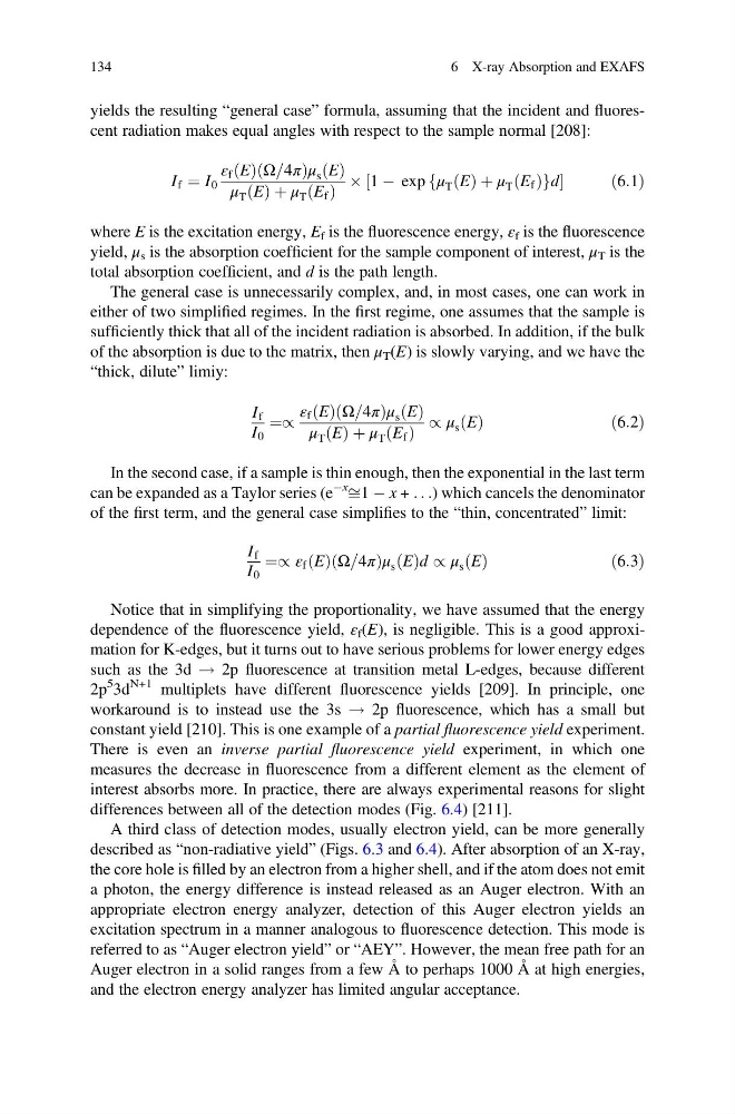
yields the resulting “general case” formula, assuming that the incident and fluorescent radiation makes equal angles with respect to the sample normal [208]:
I f ¼ I 0
ε f E
ð Þ Ω=4π
ð
Þμ s E
ð Þ
μ T E
ð Þ þ μ T E f
ð Þ
 1 À exp μ T E
ð Þ þ μ T E f
ð Þ
f
g d
½
ð 6:1Þ
where E is the excitation energy, E f is the fluorescence energy, ε f is the fluorescence
yield, μ s is the absorption coefficient for the sample component of interest, μ T is the
total absorption coefficient, and d is the path length.
The general case is unnecessarily complex, and, in most cases, one can work in
either of two simplified regimes. In the first regime, one assumes that the sample is
sufficiently thick that all of the incident radiation is absorbed. In addition, if the bulk
of the absorption is due to the matrix, then μ T (E) is slowly varying, and we have the
“thick, dilute” limiy:
I f
I 0
¼/
ε f E
ð Þ Ω=4π
ð
Þμ s E
ð Þ
μ T E
ð Þ þ μ T E f
ð Þ
/ μ s E
ð Þ
ð6:2Þ
In the second case, if a sample is thin enough, then the exponential in the last term
can be expanded as a Taylor series (e
Àx
ffi1 À x + . . .) which cancels the denominator
of the first term, and the general case simplifies to the “thin, concentrated” limit:
I f
I 0
¼/ ε f E
ð Þ Ω=4π
ð
Þμ s E
ð Þd / μ s E
ð Þ
ð6:3Þ
Notice that in simplifying the proportionality, we have assumed that the energy
dependence of the fluorescence yield, ε f (E), is negligible. This is a good approximation for K-edges, but it turns out to have serious problems for lower energy edges
such as the 3d ! 2p fluorescence at transition metal L-edges, because different
2p
5 3d
N+1 multiplets have different fluorescence yields [209]. In principle, one
workaround is to instead use the 3s ! 2p fluorescence, which has a small but
constant yield [210]. This is one example of a partial fluorescence yield experiment.
There is even an inverse partial fluorescence yield experiment, in which one
measures the decrease in fluorescence from a different element as the element of
interest absorbs more. In practice, there are always experimental reasons for slight
differences between all of the detection modes (Fig. 6.4) [211].
A third class of detection modes, usually electron yield, can be more generally
described as “non-radiative yield” (Figs. 6.3 and 6.4). After absorption of an X-ray,
the core hole is filled by an electron from a higher shell, and if the atom does not emit
a photon, the energy difference is instead released as an Auger electron. With an
appropriate electron energy analyzer, detection of this Auger electron yields an
excitation spectrum in a manner analogous to fluorescence detection. This mode is
referred to as “Auger electron yield” or “AEY”. However, the mean free path for an
Auger electron in a solid ranges from a few Å to perhaps 1000 Å at high energies,
and the electron energy analyzer has limited angular acceptance.
134
6 X-ray Absorption and EXAFS
I f ¼ I 0
ε f E
ð Þ Ω=4π
ð
Þμ s E
ð Þ
μ T E
ð Þ þ μ T E f
ð Þ
 1 À exp μ T E
ð Þ þ μ T E f
ð Þ
f
g d
½
ð 6:1Þ
where E is the excitation energy, E f is the fluorescence energy, ε f is the fluorescence
yield, μ s is the absorption coefficient for the sample component of interest, μ T is the
total absorption coefficient, and d is the path length.
The general case is unnecessarily complex, and, in most cases, one can work in
either of two simplified regimes. In the first regime, one assumes that the sample is
sufficiently thick that all of the incident radiation is absorbed. In addition, if the bulk
of the absorption is due to the matrix, then μ T (E) is slowly varying, and we have the
“thick, dilute” limiy:
I f
I 0
¼/
ε f E
ð Þ Ω=4π
ð
Þμ s E
ð Þ
μ T E
ð Þ þ μ T E f
ð Þ
/ μ s E
ð Þ
ð6:2Þ
In the second case, if a sample is thin enough, then the exponential in the last term
can be expanded as a Taylor series (e
Àx
ffi1 À x + . . .) which cancels the denominator
of the first term, and the general case simplifies to the “thin, concentrated” limit:
I f
I 0
¼/ ε f E
ð Þ Ω=4π
ð
Þμ s E
ð Þd / μ s E
ð Þ
ð6:3Þ
Notice that in simplifying the proportionality, we have assumed that the energy
dependence of the fluorescence yield, ε f (E), is negligible. This is a good approximation for K-edges, but it turns out to have serious problems for lower energy edges
such as the 3d ! 2p fluorescence at transition metal L-edges, because different
2p
5 3d
N+1 multiplets have different fluorescence yields [209]. In principle, one
workaround is to instead use the 3s ! 2p fluorescence, which has a small but
constant yield [210]. This is one example of a partial fluorescence yield experiment.
There is even an inverse partial fluorescence yield experiment, in which one
measures the decrease in fluorescence from a different element as the element of
interest absorbs more. In practice, there are always experimental reasons for slight
differences between all of the detection modes (Fig. 6.4) [211].
A third class of detection modes, usually electron yield, can be more generally
described as “non-radiative yield” (Figs. 6.3 and 6.4). After absorption of an X-ray,
the core hole is filled by an electron from a higher shell, and if the atom does not emit
a photon, the energy difference is instead released as an Auger electron. With an
appropriate electron energy analyzer, detection of this Auger electron yields an
excitation spectrum in a manner analogous to fluorescence detection. This mode is
referred to as “Auger electron yield” or “AEY”. However, the mean free path for an
Auger electron in a solid ranges from a few Å to perhaps 1000 Å at high energies,
and the electron energy analyzer has limited angular acceptance.
134
6 X-ray Absorption and EXAFS