

766
/
/
/
y
y= ax, '
/
/
/
/
/
/
/
/
c
Étude des arcs paramétrés
/
/
/
X
t--+ to
/
/
/
y
/
/
/
/
/
/
/
/
/
/
,
' ' y=ax+b
, '
X
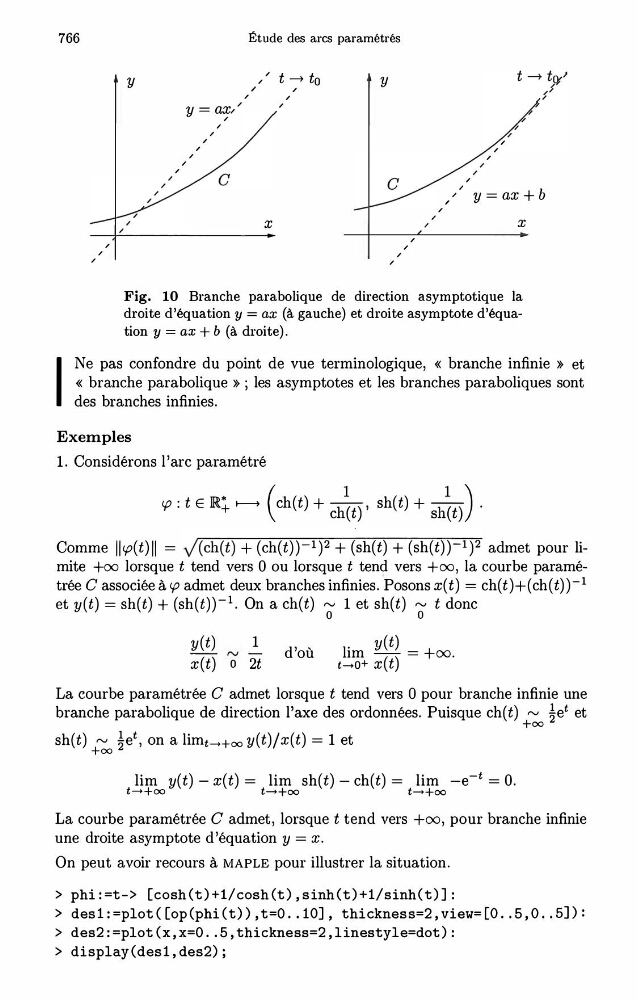
Fig. 10 Branche parabolique de direction asymptotique la
droite d'équation y= ax (à gauche) et droite asymptote d'équation y= ax + b (à droite) .
1 Ne pas confondre du point de vue terminologique, « branche infinie » et
« branche parabolique » ; les asymptotes et les branches paraboliques sont
des branches infinies.
Exemples
1. Considérons l'arc paramétré
Comme llcp(t)ll = J(ch(t) + (ch(t)) - 1 ) 2 + (sh(t) + (sh(t))- 1 ) 2 admet pour limite +oo lorsque t tend vers 0 ou lorsque t tend vers +oo, la courbe paramétrée C associée à et y(t) = sh(t) + (sh(t)) - 1 . On a ch(t) ,... ., 1 et sh(t) ,... ., t donc
0
0
y(t)
1
x(t) o 2t
d'où
. y(t)
hm -
()
= +oo.
t-+O+ X t
La courbe paramétrée C admet lorsque t tend vers 0 pour branche infinie une
branche parabolique de direction l'axe des ordonnées. Puisque ch(t) ,... ., �e t et
+oo
sh(t) ,... ., �e t , on a lim t-++oo y(t)/x(t) = 1 et
+oo
lim y(t) - x(t) = lim sh(t) - ch(t) = lim -e- t =O.
t-++oo
t-++oo
t-++oo
La courbe paramétrée C admet, lorsque t tend vers +oo, pour branche infinie
une droite asymptote d'équation y= x.
On peut avoir recours à MAPLE pour illustrer la situation.
> phi :=t-> [cosh (t)+1/cosh (t) ,sinh (t)+1/sinh(t)] :
> desi : =plot ( [op (phi (t) ) ,t=O .. 10] , thickness=2 ,view= [0 .. 5,0 .. 5]) :
> des2 : =plot (x, x=O .. 5 , thickness=2 , linestyle=dot ) :
> display (des1,des2) ;
/
/
/
y
y= ax, '
/
/
/
/
/
/
/
/
c
Étude des arcs paramétrés
/
/
/
X
t--+ to
/
/
/
y
/
/
/
/
/
/
/
/
/
/
,
' ' y=ax+b
, '
X
Fig. 10 Branche parabolique de direction asymptotique la
droite d'équation y= ax (à gauche) et droite asymptote d'équation y= ax + b (à droite) .
1 Ne pas confondre du point de vue terminologique, « branche infinie » et
« branche parabolique » ; les asymptotes et les branches paraboliques sont
des branches infinies.
Exemples
1. Considérons l'arc paramétré
Comme llcp(t)ll = J(ch(t) + (ch(t)) - 1 ) 2 + (sh(t) + (sh(t))- 1 ) 2 admet pour limite +oo lorsque t tend vers 0 ou lorsque t tend vers +oo, la courbe paramétrée C associée à et y(t) = sh(t) + (sh(t)) - 1 . On a ch(t) ,... ., 1 et sh(t) ,... ., t donc
0
0
y(t)
1
x(t) o 2t
d'où
. y(t)
hm -
()
= +oo.
t-+O+ X t
La courbe paramétrée C admet lorsque t tend vers 0 pour branche infinie une
branche parabolique de direction l'axe des ordonnées. Puisque ch(t) ,... ., �e t et
+oo
sh(t) ,... ., �e t , on a lim t-++oo y(t)/x(t) = 1 et
+oo
lim y(t) - x(t) = lim sh(t) - ch(t) = lim -e- t =O.
t-++oo
t-++oo
t-++oo
La courbe paramétrée C admet, lorsque t tend vers +oo, pour branche infinie
une droite asymptote d'équation y= x.
On peut avoir recours à MAPLE pour illustrer la situation.
> phi :=t-> [cosh (t)+1/cosh (t) ,sinh (t)+1/sinh(t)] :
> desi : =plot ( [op (phi (t) ) ,t=O .. 10] , thickness=2 ,view= [0 .. 5,0 .. 5]) :
> des2 : =plot (x, x=O .. 5 , thickness=2 , linestyle=dot ) :
> display (des1,des2) ;