

24
B. Sutcliffe and R.G. Woolley
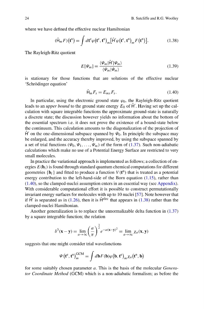
where we have defined the effective nuclear Hamiltonian
( ˆ
H m F )
t
n
=
dt
e ϕ
t
e , t
n
m
ˆ
H
ϕ
t
e , t
n
m
F
t
n
.
(1.38)
The Rayleigh-Ritz quotient
E[Ψ m ] =
Ψ m | ˆ
H |Ψ m
Ψ m |Ψ m
(1.39)
is stationary for those functions that are solutions of the effective nuclear
‘Schrödinger equation’
ˆ
H m F s = E ms F s .
(1.40)
In particular, using the electronic ground state ϕ 0 , the Rayleigh-Ritz quotient
leads to an upper bound to the ground state energy E 0 of ˆ
H . Having set up the calculation with square integrable functions the approximate ground-state is naturally
a discrete state; the discussion however yields no information about the bottom of
the essential spectrum i.e. it does not prove the existence of a bound-state below
the continuum. This calculation amounts to the diagonalization of the projection of
ˆ
H on the one-dimensional subspace spanned by Ψ 0 . In principle the subspace may
be enlarged, and the accuracy thereby improved, by using the subspace spanned by
a set of trial functions (Ψ 0 , Ψ 1 , . . . , Ψ m ) of the form of (1.37). Such non-adiabatic
calculations which make no use of a Potential Energy Surface are restricted to very
small molecules.
In practice the variational approach is implemented as follows; a collection of energies E(b i ) is found through standard quantum chemical computations for different
geometries {b i } and fitted to produce a function V (t n ) that is treated as a potential
energy contribution to the left-hand-side of the Born equation (1.15), rather than
(1.40), so the clamped-nuclei assumption enters in an essential way (see Appendix).
With considerable computational effort it is possible to construct permutationally
invariant energy surfaces for molecules with up to 10 nuclei [57]. Note however that
if ˆ
H is separated as in (1.26), then it is ˆ
H elec that appears in (1.38) rather than the
clamped-nuclei Hamiltonian.
Another generalization is to replace the unnormalizable delta function in (1.37)
by a square integrable function; the relation
δ
3 (x − y) = lim
a→∞
a
π
3
2
e
−a(x−y) 2 ≡ lim
a→∞
χ a (x, y)
suggests that one might consider trial wavefunctions
Ψ
t
e , t
n
GCM
m
=
dbF (b)ϕ
b, t
e
m
χ a
t
n , b
for some suitably chosen parameter a. This is the basis of the molecular Generator Coordinate Method (GCM) which is a non-adiabatic formalism; as before the
B. Sutcliffe and R.G. Woolley
where we have defined the effective nuclear Hamiltonian
( ˆ
H m F )
t
n
=
dt
e ϕ
t
e , t
n
m
ˆ
H
ϕ
t
e , t
n
m
F
t
n
.
(1.38)
The Rayleigh-Ritz quotient
E[Ψ m ] =
Ψ m | ˆ
H |Ψ m
Ψ m |Ψ m
(1.39)
is stationary for those functions that are solutions of the effective nuclear
‘Schrödinger equation’
ˆ
H m F s = E ms F s .
(1.40)
In particular, using the electronic ground state ϕ 0 , the Rayleigh-Ritz quotient
leads to an upper bound to the ground state energy E 0 of ˆ
H . Having set up the calculation with square integrable functions the approximate ground-state is naturally
a discrete state; the discussion however yields no information about the bottom of
the essential spectrum i.e. it does not prove the existence of a bound-state below
the continuum. This calculation amounts to the diagonalization of the projection of
ˆ
H on the one-dimensional subspace spanned by Ψ 0 . In principle the subspace may
be enlarged, and the accuracy thereby improved, by using the subspace spanned by
a set of trial functions (Ψ 0 , Ψ 1 , . . . , Ψ m ) of the form of (1.37). Such non-adiabatic
calculations which make no use of a Potential Energy Surface are restricted to very
small molecules.
In practice the variational approach is implemented as follows; a collection of energies E(b i ) is found through standard quantum chemical computations for different
geometries {b i } and fitted to produce a function V (t n ) that is treated as a potential
energy contribution to the left-hand-side of the Born equation (1.15), rather than
(1.40), so the clamped-nuclei assumption enters in an essential way (see Appendix).
With considerable computational effort it is possible to construct permutationally
invariant energy surfaces for molecules with up to 10 nuclei [57]. Note however that
if ˆ
H is separated as in (1.26), then it is ˆ
H elec that appears in (1.38) rather than the
clamped-nuclei Hamiltonian.
Another generalization is to replace the unnormalizable delta function in (1.37)
by a square integrable function; the relation
δ
3 (x − y) = lim
a→∞
a
π
3
2
e
−a(x−y) 2 ≡ lim
a→∞
χ a (x, y)
suggests that one might consider trial wavefunctions
Ψ
t
e , t
n
GCM
m
=
dbF (b)ϕ
b, t
e
m
χ a
t
n , b
for some suitably chosen parameter a. This is the basis of the molecular Generator Coordinate Method (GCM) which is a non-adiabatic formalism; as before the