

18 On Converse Piezoelectricity
341
to the infinite periodic chain calculations with ˜
n equal to 0 and −2. The important
point is that the finite chain and infinite periodic chain results lie on top of one
another, which means that the properties do coincide. Second, different values of
˜
n, or Q R , lead to different results. For the infinite periodic system the integer ˜
n
exactly mimics the effect of the terminal charge, Q R , for the large finite system.
We hasten to add that the calculations are several orders of magnitude faster for
the former system than for the latter. Finally, the variation in a, as a function of E,
is what causes all other properties to depend upon the terminal charge. This was
also demonstrated in [8, 16], where it was shown that the dependence upon terminal
charge is eliminated by keeping a fixed.
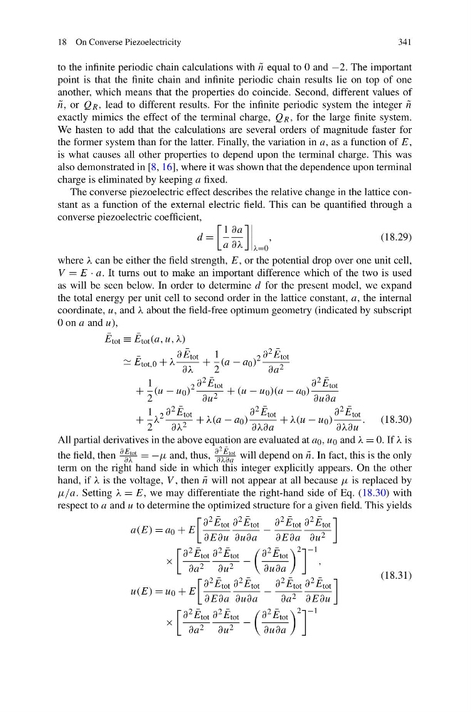
The converse piezoelectric effect describes the relative change in the lattice constant as a function of the external electric field. This can be quantified through a
converse piezoelectric coefficient,
d =
1
a
∂a
∂λ
λ=0
,
(18.29)
where λ can be either the field strength, E, or the potential drop over one unit cell,
V = E · a. It turns out to make an important difference which of the two is used
as will be seen below. In order to determine d for the present model, we expand
the total energy per unit cell to second order in the lattice constant, a, the internal
coordinate, u, and λ about the field-free optimum geometry (indicated by subscript
0 on a and u),
¯
E tot ≡ ¯
E tot (a, u, λ)
¯
E tot,0 + λ
∂ ¯
E tot
∂λ
+
1
2
(a − a 0 )
2 ∂ 2 ¯
E tot
∂a 2
+
1
2
(u − u 0 )
2 ∂ 2 ¯
E tot
∂u 2 + (u − u 0 )(a − a 0 )
∂ 2 ¯
E tot
∂u∂a
+
1
2
λ
2 ∂ 2 ¯
E tot
∂λ 2 + λ(a − a 0 )
∂ 2 ¯
E tot
∂λ∂a
+ λ(u − u 0 )
∂ 2 ¯
E tot
∂λ∂u
. (18.30)
All partial derivatives in the above equation are evaluated at a 0 , u 0 and λ = 0. If λ is
the field, then
∂E tot
∂λ = −μ and, thus,
∂ 2 ¯
E tot
∂λ∂a will depend on ˜
n. In fact, this is the only
term on the right hand side in which this integer explicitly appears. On the other
hand, if λ is the voltage, V , then ˜
n will not appear at all because μ is replaced by
μ/a. Setting λ = E, we may differentiate the right-hand side of Eq. (18.30) with
respect to a and u to determine the optimized structure for a given field. This yields
a(E) = a 0 + E
∂ 2 ¯
E tot
∂E∂u
∂ 2 ¯
E tot
∂u∂a
−
∂ 2 ¯
E tot
∂E∂a
∂ 2 ¯
E tot
∂u 2
×
∂ 2 ¯
E tot
∂a 2
∂ 2 ¯
E tot
∂u 2 −
∂ 2 ¯
E tot
∂u∂a
2 −1
,
u(E) = u 0 + E
∂ 2 ¯
E tot
∂E∂a
∂ 2 ¯
E tot
∂u∂a
−
∂ 2 ¯
E tot
∂a 2
∂ 2 ¯
E tot
∂E∂u
×
∂ 2 ¯
E tot
∂a 2
∂ 2 ¯
E tot
∂u 2 −
∂ 2 ¯
E tot
∂u∂a
2 −1
(18.31)
341
to the infinite periodic chain calculations with ˜
n equal to 0 and −2. The important
point is that the finite chain and infinite periodic chain results lie on top of one
another, which means that the properties do coincide. Second, different values of
˜
n, or Q R , lead to different results. For the infinite periodic system the integer ˜
n
exactly mimics the effect of the terminal charge, Q R , for the large finite system.
We hasten to add that the calculations are several orders of magnitude faster for
the former system than for the latter. Finally, the variation in a, as a function of E,
is what causes all other properties to depend upon the terminal charge. This was
also demonstrated in [8, 16], where it was shown that the dependence upon terminal
charge is eliminated by keeping a fixed.
The converse piezoelectric effect describes the relative change in the lattice constant as a function of the external electric field. This can be quantified through a
converse piezoelectric coefficient,
d =
1
a
∂a
∂λ
λ=0
,
(18.29)
where λ can be either the field strength, E, or the potential drop over one unit cell,
V = E · a. It turns out to make an important difference which of the two is used
as will be seen below. In order to determine d for the present model, we expand
the total energy per unit cell to second order in the lattice constant, a, the internal
coordinate, u, and λ about the field-free optimum geometry (indicated by subscript
0 on a and u),
¯
E tot ≡ ¯
E tot (a, u, λ)
¯
E tot,0 + λ
∂ ¯
E tot
∂λ
+
1
2
(a − a 0 )
2 ∂ 2 ¯
E tot
∂a 2
+
1
2
(u − u 0 )
2 ∂ 2 ¯
E tot
∂u 2 + (u − u 0 )(a − a 0 )
∂ 2 ¯
E tot
∂u∂a
+
1
2
λ
2 ∂ 2 ¯
E tot
∂λ 2 + λ(a − a 0 )
∂ 2 ¯
E tot
∂λ∂a
+ λ(u − u 0 )
∂ 2 ¯
E tot
∂λ∂u
. (18.30)
All partial derivatives in the above equation are evaluated at a 0 , u 0 and λ = 0. If λ is
the field, then
∂E tot
∂λ = −μ and, thus,
∂ 2 ¯
E tot
∂λ∂a will depend on ˜
n. In fact, this is the only
term on the right hand side in which this integer explicitly appears. On the other
hand, if λ is the voltage, V , then ˜
n will not appear at all because μ is replaced by
μ/a. Setting λ = E, we may differentiate the right-hand side of Eq. (18.30) with
respect to a and u to determine the optimized structure for a given field. This yields
a(E) = a 0 + E
∂ 2 ¯
E tot
∂E∂u
∂ 2 ¯
E tot
∂u∂a
−
∂ 2 ¯
E tot
∂E∂a
∂ 2 ¯
E tot
∂u 2
×
∂ 2 ¯
E tot
∂a 2
∂ 2 ¯
E tot
∂u 2 −
∂ 2 ¯
E tot
∂u∂a
2 −1
,
u(E) = u 0 + E
∂ 2 ¯
E tot
∂E∂a
∂ 2 ¯
E tot
∂u∂a
−
∂ 2 ¯
E tot
∂a 2
∂ 2 ¯
E tot
∂E∂u
×
∂ 2 ¯
E tot
∂a 2
∂ 2 ¯
E tot
∂u 2 −
∂ 2 ¯
E tot
∂u∂a
2 −1
(18.31)