

342
M. Springborg et al.
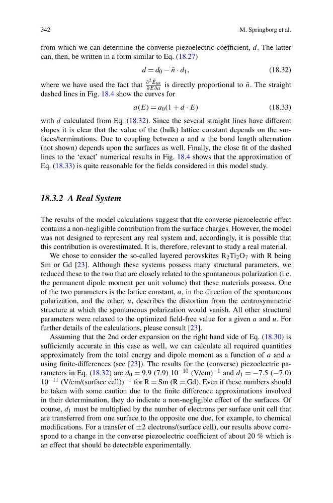
from which we can determine the converse piezoelectric coefficient, d. The latter
can, then, be written in a form similar to Eq. (18.27)
d = d 0 − ˜
n · d 1 ,
(18.32)
where we have used the fact that
∂ 2 ¯
E tot
∂E∂a is directly proportional to ˜
n. The straight
dashed lines in Fig. 18.4 show the curves for
a(E) = a 0 (1 + d · E)
(18.33)
with d calculated from Eq. (18.32). Since the several straight lines have different
slopes it is clear that the value of the (bulk) lattice constant depends on the surfaces/terminations. Due to coupling between a and u the bond length alternation
(not shown) depends upon the surfaces as well. Finally, the close fit of the dashed
lines to the ‘exact’ numerical results in Fig. 18.4 shows that the approximation of
Eq. (18.33) is quite reasonable for the fields considered in this model study.
18.3.2 A Real System
The results of the model calculations suggest that the converse piezoelectric effect
contains a non-negligible contribution from the surface charges. However, the model
was not designed to represent any real system and, accordingly, it is possible that
this contribution is overestimated. It is, therefore, relevant to study a real material.
We chose to consider the so-called layered perovskites R 2 Ti 2 O 7 with R being
Sm or Gd [23]. Although these systems possess many structural parameters, we
reduced these to the two that are closely related to the spontaneous polarization (i.e.
the permanent dipole moment per unit volume) that these materials possess. One
of the two parameters is the lattice constant, a, in the direction of the spontaneous
polarization, and the other, u, describes the distortion from the centrosymmetric
structure at which the spontaneous polarization would vanish. All other structural
parameters were relaxed to the optimized field-free value for a given a and u. For
further details of the calculations, please consult [23].
Assuming that the 2nd order expansion on the right hand side of Eq. (18.30) is
sufficiently accurate in this case as well, we can calculate all required quantities
approximately from the total energy and dipole moment as a function of a and u
using finite-differences (see [23]). The results for the (converse) piezoelectric parameters in Eq. (18.32) are d 0 = 9.9 (7.9) 10 −10 (V/cm) −1 and d 1 = −7.5 (−7.0)
10 −11 (V/cm/(surface cell)) −1 for R = Sm (R = Gd). Even if these numbers should
be taken with some caution due to the finite difference approximations involved
in their determination, they do indicate a non-negligible effect of the surfaces. Of
course, d 1 must be multiplied by the number of electrons per surface unit cell that
are transferred from one surface to the opposite one due, for example, to chemical
modifications. For a transfer of ±2 electrons/(surface cell), our results above correspond to a change in the converse piezoelectric coefficient of about 20 % which is
an effect that should be detectable experimentally.
M. Springborg et al.
from which we can determine the converse piezoelectric coefficient, d. The latter
can, then, be written in a form similar to Eq. (18.27)
d = d 0 − ˜
n · d 1 ,
(18.32)
where we have used the fact that
∂ 2 ¯
E tot
∂E∂a is directly proportional to ˜
n. The straight
dashed lines in Fig. 18.4 show the curves for
a(E) = a 0 (1 + d · E)
(18.33)
with d calculated from Eq. (18.32). Since the several straight lines have different
slopes it is clear that the value of the (bulk) lattice constant depends on the surfaces/terminations. Due to coupling between a and u the bond length alternation
(not shown) depends upon the surfaces as well. Finally, the close fit of the dashed
lines to the ‘exact’ numerical results in Fig. 18.4 shows that the approximation of
Eq. (18.33) is quite reasonable for the fields considered in this model study.
18.3.2 A Real System
The results of the model calculations suggest that the converse piezoelectric effect
contains a non-negligible contribution from the surface charges. However, the model
was not designed to represent any real system and, accordingly, it is possible that
this contribution is overestimated. It is, therefore, relevant to study a real material.
We chose to consider the so-called layered perovskites R 2 Ti 2 O 7 with R being
Sm or Gd [23]. Although these systems possess many structural parameters, we
reduced these to the two that are closely related to the spontaneous polarization (i.e.
the permanent dipole moment per unit volume) that these materials possess. One
of the two parameters is the lattice constant, a, in the direction of the spontaneous
polarization, and the other, u, describes the distortion from the centrosymmetric
structure at which the spontaneous polarization would vanish. All other structural
parameters were relaxed to the optimized field-free value for a given a and u. For
further details of the calculations, please consult [23].
Assuming that the 2nd order expansion on the right hand side of Eq. (18.30) is
sufficiently accurate in this case as well, we can calculate all required quantities
approximately from the total energy and dipole moment as a function of a and u
using finite-differences (see [23]). The results for the (converse) piezoelectric parameters in Eq. (18.32) are d 0 = 9.9 (7.9) 10 −10 (V/cm) −1 and d 1 = −7.5 (−7.0)
10 −11 (V/cm/(surface cell)) −1 for R = Sm (R = Gd). Even if these numbers should
be taken with some caution due to the finite difference approximations involved
in their determination, they do indicate a non-negligible effect of the surfaces. Of
course, d 1 must be multiplied by the number of electrons per surface unit cell that
are transferred from one surface to the opposite one due, for example, to chemical
modifications. For a transfer of ±2 electrons/(surface cell), our results above correspond to a change in the converse piezoelectric coefficient of about 20 % which is
an effect that should be detectable experimentally.