

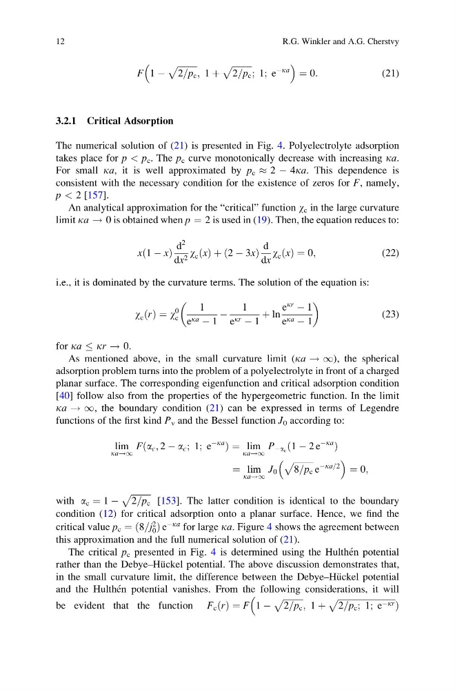
F 1 À
ffiffiffiffiffiffiffiffiffi
2=p c
p
; 1 þ
ffiffiffiffiffiffiffiffiffi
2=p c
p
; 1; e
Àka
¼ 0:
(21)
3.2.1 Critical Adsorption
The numerical solution of (21) is presented in Fig. 4. Polyelectrolyte adsorption
takes place for p < p c . The p c curve monotonically decrease with increasing ka.
For small ka, it is well approximated by p c % 2 À 4ka. This dependence is
consistent with the necessary condition for the existence of zeros for F, namely,
p < 2 [157].
An analytical approximation for the “critical” function w c in the large curvature
limit ka ! 0 is obtained when p ¼ 2 is used in (19). Then, the equation reduces to:
xð1 À xÞ
d
2
dx 2 w c ðxÞ þ ð2 À 3xÞ
d
dx
w c ðxÞ ¼ 0;
(22)
i.e., it is dominated by the curvature terms. The solution of the equation is:
w c ðrÞ ¼ w
0
c
1
e ka À 1
À
1
e kr À 1
þ ln
e
kr
À 1
e ka À 1
(23)
for ka kr ! 0.
As mentioned above, in the small curvature limit (ka ! 1), the spherical
adsorption problem turns into the problem of a polyelectrolyte in front of a charged
planar surface. The corresponding eigenfunction and critical adsorption condition
[40] follow also from the properties of the hypergeometric function. In the limit
ka ! 1, the boundary condition (21) can be expressed in terms of Legendre
functions of the first kind P n and the Bessel function J 0 according to:
lim
ka!1
Fða c ; 2 À a c ; 1; e
Àka
Þ ¼ lim
ka!1
P Àa c ð1 À 2 e
Àka
Þ
¼ lim
ka!1
J 0
ffiffiffiffiffiffiffiffiffi
8=p c
p
e
Àka=2
¼ 0;
with a c ¼ 1 À
ffiffiffiffiffiffiffiffiffi
2=p c
p
[153]. The latter condition is identical to the boundary
condition (12) for critical adsorption onto a planar surface. Hence, we find the
critical value p c ¼ ð8=j
2
0 Þ e
Àka for large ka. Figure 4 shows the agreement between
this approximation and the full numerical solution of (21).
The critical p c presented in Fig. 4 is determined using the Hulthe ´n potential
rather than the Debye–Hu ¨ckel potential. The above discussion demonstrates that,
in the small curvature limit, the difference between the Debye–Hu ¨ckel potential
and the Hulthe ´n potential vanishes. From the following considerations, it will
be evident that the function F c ðrÞ ¼ F 1 À
ffiffiffiffiffiffiffiffiffi
2=p c
p
; 1 þ
ffiffiffiffiffiffiffiffiffiffiffiffiffiffiffiffiffiffiffiffiffiffiffiffiffiffi ffi
2=p c ; 1; e Àkr
p
Þ
12
R.G. Winkler and A.G. Cherstvy
ffiffiffiffiffiffiffiffiffi
2=p c
p
; 1 þ
ffiffiffiffiffiffiffiffiffi
2=p c
p
; 1; e
Àka
¼ 0:
(21)
3.2.1 Critical Adsorption
The numerical solution of (21) is presented in Fig. 4. Polyelectrolyte adsorption
takes place for p < p c . The p c curve monotonically decrease with increasing ka.
For small ka, it is well approximated by p c % 2 À 4ka. This dependence is
consistent with the necessary condition for the existence of zeros for F, namely,
p < 2 [157].
An analytical approximation for the “critical” function w c in the large curvature
limit ka ! 0 is obtained when p ¼ 2 is used in (19). Then, the equation reduces to:
xð1 À xÞ
d
2
dx 2 w c ðxÞ þ ð2 À 3xÞ
d
dx
w c ðxÞ ¼ 0;
(22)
i.e., it is dominated by the curvature terms. The solution of the equation is:
w c ðrÞ ¼ w
0
c
1
e ka À 1
À
1
e kr À 1
þ ln
e
kr
À 1
e ka À 1
(23)
for ka kr ! 0.
As mentioned above, in the small curvature limit (ka ! 1), the spherical
adsorption problem turns into the problem of a polyelectrolyte in front of a charged
planar surface. The corresponding eigenfunction and critical adsorption condition
[40] follow also from the properties of the hypergeometric function. In the limit
ka ! 1, the boundary condition (21) can be expressed in terms of Legendre
functions of the first kind P n and the Bessel function J 0 according to:
lim
ka!1
Fða c ; 2 À a c ; 1; e
Àka
Þ ¼ lim
ka!1
P Àa c ð1 À 2 e
Àka
Þ
¼ lim
ka!1
J 0
ffiffiffiffiffiffiffiffiffi
8=p c
p
e
Àka=2
¼ 0;
with a c ¼ 1 À
ffiffiffiffiffiffiffiffiffi
2=p c
p
[153]. The latter condition is identical to the boundary
condition (12) for critical adsorption onto a planar surface. Hence, we find the
critical value p c ¼ ð8=j
2
0 Þ e
Àka for large ka. Figure 4 shows the agreement between
this approximation and the full numerical solution of (21).
The critical p c presented in Fig. 4 is determined using the Hulthe ´n potential
rather than the Debye–Hu ¨ckel potential. The above discussion demonstrates that,
in the small curvature limit, the difference between the Debye–Hu ¨ckel potential
and the Hulthe ´n potential vanishes. From the following considerations, it will
be evident that the function F c ðrÞ ¼ F 1 À
ffiffiffiffiffiffiffiffiffi
2=p c
p
; 1 þ
ffiffiffiffiffiffiffiffiffiffiffiffiffiffiffiffiffiffiffiffiffiffiffiffiffiffi ffi
2=p c ; 1; e Àkr
p
Þ
12
R.G. Winkler and A.G. Cherstvy