

Summing up, the external contribution to the energetic density of states in P3HT
was shown to be intimately connected to paracrystallinity along the π-stacking
direction, with the energetic disorder σ linearly related to the amplitude of
backbone–backbone distance fluctuations, and the mean of the backbone–backbone
distance distribution analogously related to the average site energy hUi.
4.5 Charge Mobility
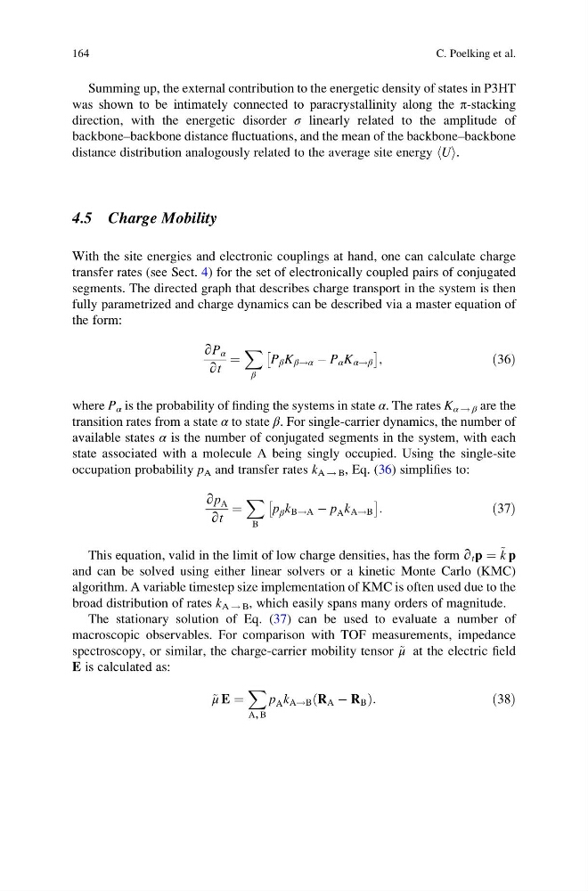
With the site energies and electronic couplings at hand, one can calculate charge
transfer rates (see Sect. 4) for the set of electronically coupled pairs of conjugated
segments. The directed graph that describes charge transport in the system is then
fully parametrized and charge dynamics can be described via a master equation of
the form:
∂P α
∂t
¼
X
β
P β K β!α À P α K α!β
Â
Ã
,
ð36Þ
where P α is the probability of finding the systems in state α. The rates K α ! β are the
transition rates from a state α to state β. For single-carrier dynamics, the number of
available states α is the number of conjugated segments in the system, with each
state associated with a molecule A being singly occupied. Using the single-site
occupation probability p A and transfer rates k A ! B , Eq. (36) simplifies to:
∂p A
∂t
¼
X
B
p β k B!A À p A k A!B
Â
à :
ð37Þ
This equation, valid in the limit of low charge densities, has the form ∂ t p ¼ ~ k p
and can be solved using either linear solvers or a kinetic Monte Carlo (KMC)
algorithm. A variable timestep size implementation of KMC is often used due to the
broad distribution of rates k A ! B , which easily spans many orders of magnitude.
The stationary solution of Eq. (37) can be used to evaluate a number of
macroscopic observables. For comparison with TOF measurements, impedance
spectroscopy, or similar, the charge-carrier mobility tensor ~
μ at the electric field
E is calculated as:
~
μ E ¼
X
A, B
p A k A!B R A À R B
ð
Þ :
ð38Þ
164
C. Poelking et al.
was shown to be intimately connected to paracrystallinity along the π-stacking
direction, with the energetic disorder σ linearly related to the amplitude of
backbone–backbone distance fluctuations, and the mean of the backbone–backbone
distance distribution analogously related to the average site energy hUi.
4.5 Charge Mobility
With the site energies and electronic couplings at hand, one can calculate charge
transfer rates (see Sect. 4) for the set of electronically coupled pairs of conjugated
segments. The directed graph that describes charge transport in the system is then
fully parametrized and charge dynamics can be described via a master equation of
the form:
∂P α
∂t
¼
X
β
P β K β!α À P α K α!β
Â
Ã
,
ð36Þ
where P α is the probability of finding the systems in state α. The rates K α ! β are the
transition rates from a state α to state β. For single-carrier dynamics, the number of
available states α is the number of conjugated segments in the system, with each
state associated with a molecule A being singly occupied. Using the single-site
occupation probability p A and transfer rates k A ! B , Eq. (36) simplifies to:
∂p A
∂t
¼
X
B
p β k B!A À p A k A!B
Â
à :
ð37Þ
This equation, valid in the limit of low charge densities, has the form ∂ t p ¼ ~ k p
and can be solved using either linear solvers or a kinetic Monte Carlo (KMC)
algorithm. A variable timestep size implementation of KMC is often used due to the
broad distribution of rates k A ! B , which easily spans many orders of magnitude.
The stationary solution of Eq. (37) can be used to evaluate a number of
macroscopic observables. For comparison with TOF measurements, impedance
spectroscopy, or similar, the charge-carrier mobility tensor ~
μ at the electric field
E is calculated as:
~
μ E ¼
X
A, B
p A k A!B R A À R B
ð
Þ :
ð38Þ
164
C. Poelking et al.