

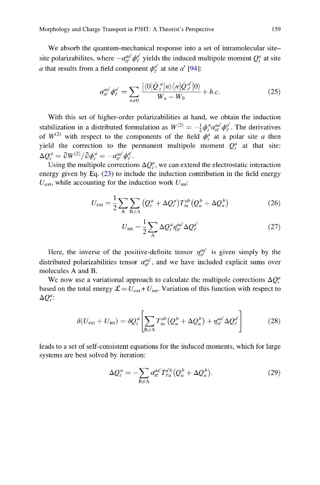
We absorb the quantum-mechanical response into a set of intramolecular site–
site polarizabilites, where Àα
aa
0
tt 0 ϕ
a
0
t 0 yields the induced multipole moment Q
a
t at site
a that results from a field component ϕ
a
0
t 0 at site a
0 [94]:
α
aa
0
tt 0 ϕ
a
0
t 0 ¼
X
n6 ¼0
0
h
^
Q
a
t
ni n
^
Q
a
0
t 0
0i
W n À W 0
þ h:c:
ð25Þ
With this set of higher-order polarizabilities at hand, we obtain the induction
stabilization in a distributed formulation as W
2
ð Þ
¼ À
1
2 ϕ
a
t α
aa
0
tt 0 ϕ
a
0
t 0 . The derivatives
of W
(2) with respect to the components of the field ϕ
a
t at a polar site a then
yield the correction to the permanent multipole moment Q
a
t at that site:
ΔQ
a
t ¼ ∂W
2
ð Þ
=∂ϕ
a
t ¼ Àα
aa
0
tt 0 ϕ
a
0
t 0 .
Using the multipole corrections ΔQ
a
t , we can extend the electrostatic interaction
energy given by Eq. (23) to include the induction contribution in the field energy
U ext , while accounting for the induction work U int :
U ext ¼
1
2
X
A
X
B6 ¼A
Q
a
t þ ΔQ
a
t
À
Á
T
ab
tu Q
b
u þ ΔQ
b
u
À
Á
ð26Þ
U int ¼
1
2
X
A
ΔQ
a
t η
aa
0
tt 0 ΔQ
a
0
t 0
ð27Þ
Here, the inverse of the positive-definite tensor η
aa
0
tt 0 is given simply by the
distributed polarizabilities tensor α
aa
0
tt 0 , and we have included explicit sums over
molecules A and B.
We now use a variational approach to calculate the multipole corrections ΔQ
a
t
based on the total energy ℒ ¼ U ext + U int . Variation of this function with respect to
ΔQ
a
t :
δ U ext þ U int
ð
Þ¼δQ
a
t
X
B6 ¼A
T
ab
tu Q
b
u þ ΔQ
b
u
À
Á þ η
aa
0
tt 0 ΔQ
a
0
t 0
"
#
ð28Þ
leads to a set of self-consistent equations for the induced moments, which for large
systems are best solved by iteration:
ΔQ
a
t ¼ À
X
B6 ¼A
α
aa
0
tt 0 T
a
0 b
t 0 u Q
b
u þ ΔQ
b
u
À
Á :
ð29Þ
Morphology and Charge Transport in P3HT: A Theorist’s Perspective
159
site polarizabilites, where Àα
aa
0
tt 0 ϕ
a
0
t 0 yields the induced multipole moment Q
a
t at site
a that results from a field component ϕ
a
0
t 0 at site a
0 [94]:
α
aa
0
tt 0 ϕ
a
0
t 0 ¼
X
n6 ¼0
0
h
^
Q
a
t
ni n
^
Q
a
0
t 0
0i
W n À W 0
þ h:c:
ð25Þ
With this set of higher-order polarizabilities at hand, we obtain the induction
stabilization in a distributed formulation as W
2
ð Þ
¼ À
1
2 ϕ
a
t α
aa
0
tt 0 ϕ
a
0
t 0 . The derivatives
of W
(2) with respect to the components of the field ϕ
a
t at a polar site a then
yield the correction to the permanent multipole moment Q
a
t at that site:
ΔQ
a
t ¼ ∂W
2
ð Þ
=∂ϕ
a
t ¼ Àα
aa
0
tt 0 ϕ
a
0
t 0 .
Using the multipole corrections ΔQ
a
t , we can extend the electrostatic interaction
energy given by Eq. (23) to include the induction contribution in the field energy
U ext , while accounting for the induction work U int :
U ext ¼
1
2
X
A
X
B6 ¼A
Q
a
t þ ΔQ
a
t
À
Á
T
ab
tu Q
b
u þ ΔQ
b
u
À
Á
ð26Þ
U int ¼
1
2
X
A
ΔQ
a
t η
aa
0
tt 0 ΔQ
a
0
t 0
ð27Þ
Here, the inverse of the positive-definite tensor η
aa
0
tt 0 is given simply by the
distributed polarizabilities tensor α
aa
0
tt 0 , and we have included explicit sums over
molecules A and B.
We now use a variational approach to calculate the multipole corrections ΔQ
a
t
based on the total energy ℒ ¼ U ext + U int . Variation of this function with respect to
ΔQ
a
t :
δ U ext þ U int
ð
Þ¼δQ
a
t
X
B6 ¼A
T
ab
tu Q
b
u þ ΔQ
b
u
À
Á þ η
aa
0
tt 0 ΔQ
a
0
t 0
"
#
ð28Þ
leads to a set of self-consistent equations for the induced moments, which for large
systems are best solved by iteration:
ΔQ
a
t ¼ À
X
B6 ¼A
α
aa
0
tt 0 T
a
0 b
t 0 u Q
b
u þ ΔQ
b
u
À
Á :
ð29Þ
Morphology and Charge Transport in P3HT: A Theorist’s Perspective
159