

98
4 Four-Dimensional Superfield Supersymmetry
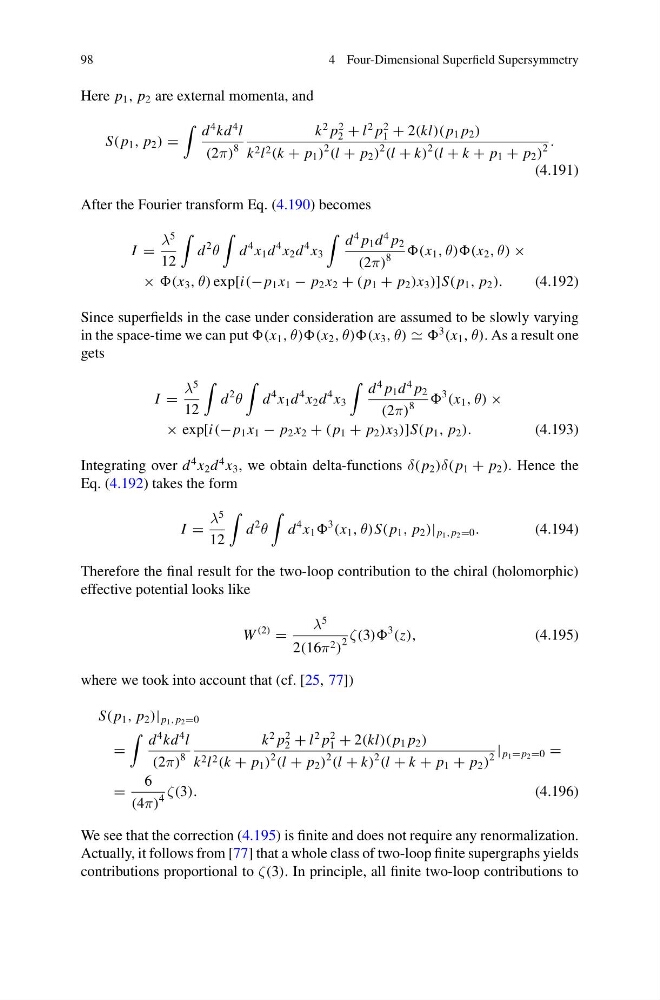
Here p 1 , p 2 are external momenta, and
S( p 1 , p 2 ) =
d
4 kd
4 l
(2π)
8
k
2 p
2
2 + l
2 p
2
1 + 2(kl)( p 1 p 2 )
k 2 l 2 (k + p 1 )
2
(l + p 2 )
2
(l + k)
2
(l + k + p 1 + p 2 )
2
.
(4.191)
After the Fourier transform Eq. (4.190) becomes
I =
λ
5
12
d
2
θ
d
4 x 1 d
4 x 2 d
4 x 3
d
4 p 1 d
4 p 2
(2π)
8
(x 1 , θ))(x 2 , θ) ×
× (x 3 , θ) exp[i(− p 1 x 1 − p 2 x 2 + ( p 1 + p 2 )x 3 )]S( p 1 , p 2 ).
(4.192)
Since superfields in the case under consideration are assumed to be slowly varying
in the space-time we can put (x 1 , θ))(x 2 , θ))(x 3 , θ)
3
(x 1 , θ). As a result one
gets
I =
λ
5
12
d
2
θ
d
4 x 1 d
4 x 2 d
4 x 3
d
4 p 1 d
4 p 2
(2π)
8
3
(x 1 , θ) ×
× exp[i(− p 1 x 1 − p 2 x 2 + ( p 1 + p 2 )x 3 )]S( p 1 , p 2 ).
(4.193)
Integrating over d
4 x 2 d
4 x 3 , we obtain delta-functions δ( p 2 )δ( p 1 + p 2 ). Hence the
Eq. (4.192) takes the form
I =
λ
5
12
d
2
θ
d
4 x 1
3
(x 1 , θ)S( p 1 , p 2 )| p 1 , p 2 =0 .
(4.194)
Therefore the final result for the two-loop contribution to the chiral (holomorphic)
effective potential looks like
W
(2)
=
λ
5
2(16π 2 )
2
ζ(3))
3
(z),
(4.195)
where we took into account that (cf. [25, 77])
S( p 1 , p 2 )| p 1 , p 2 =0
=
d
4 kd
4 l
(2π)
8
k
2 p
2
2 + l
2 p
2
1 + 2(kl)( p 1 p 2 )
k 2 l 2 (k + p 1 )
2
(l + p 2 )
2
(l + k)
2
(l + k + p 1 + p 2 )
2
| p 1 = p 2 =0 =
=
6
(4π)
4
ζ(3).
(4.196)
We see that the correction (4.195) is finite and does not require any renormalization.
Actually, it follows from [77] that a whole class of two-loop finite supergraphs yields
contributions proportional to ζ(3). In principle, all finite two-loop contributions to
4 Four-Dimensional Superfield Supersymmetry
Here p 1 , p 2 are external momenta, and
S( p 1 , p 2 ) =
d
4 kd
4 l
(2π)
8
k
2 p
2
2 + l
2 p
2
1 + 2(kl)( p 1 p 2 )
k 2 l 2 (k + p 1 )
2
(l + p 2 )
2
(l + k)
2
(l + k + p 1 + p 2 )
2
.
(4.191)
After the Fourier transform Eq. (4.190) becomes
I =
λ
5
12
d
2
θ
d
4 x 1 d
4 x 2 d
4 x 3
d
4 p 1 d
4 p 2
(2π)
8
(x 1 , θ))(x 2 , θ) ×
× (x 3 , θ) exp[i(− p 1 x 1 − p 2 x 2 + ( p 1 + p 2 )x 3 )]S( p 1 , p 2 ).
(4.192)
Since superfields in the case under consideration are assumed to be slowly varying
in the space-time we can put (x 1 , θ))(x 2 , θ))(x 3 , θ)
3
(x 1 , θ). As a result one
gets
I =
λ
5
12
d
2
θ
d
4 x 1 d
4 x 2 d
4 x 3
d
4 p 1 d
4 p 2
(2π)
8
3
(x 1 , θ) ×
× exp[i(− p 1 x 1 − p 2 x 2 + ( p 1 + p 2 )x 3 )]S( p 1 , p 2 ).
(4.193)
Integrating over d
4 x 2 d
4 x 3 , we obtain delta-functions δ( p 2 )δ( p 1 + p 2 ). Hence the
Eq. (4.192) takes the form
I =
λ
5
12
d
2
θ
d
4 x 1
3
(x 1 , θ)S( p 1 , p 2 )| p 1 , p 2 =0 .
(4.194)
Therefore the final result for the two-loop contribution to the chiral (holomorphic)
effective potential looks like
W
(2)
=
λ
5
2(16π 2 )
2
ζ(3))
3
(z),
(4.195)
where we took into account that (cf. [25, 77])
S( p 1 , p 2 )| p 1 , p 2 =0
=
d
4 kd
4 l
(2π)
8
k
2 p
2
2 + l
2 p
2
1 + 2(kl)( p 1 p 2 )
k 2 l 2 (k + p 1 )
2
(l + p 2 )
2
(l + k)
2
(l + k + p 1 + p 2 )
2
| p 1 = p 2 =0 =
=
6
(4π)
4
ζ(3).
(4.196)
We see that the correction (4.195) is finite and does not require any renormalization.
Actually, it follows from [77] that a whole class of two-loop finite supergraphs yields
contributions proportional to ζ(3). In principle, all finite two-loop contributions to