

4.8 The Wess-Zumino Model and a Problem of the Chiral Effective Potential
97
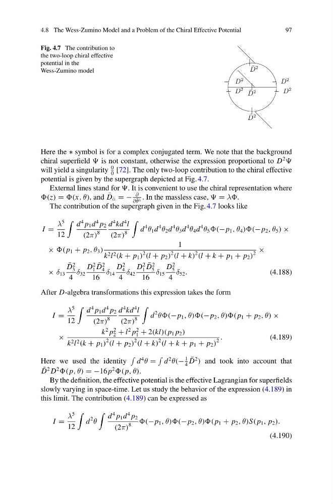
Fig. 4.7 The contribution to
the two-loop chiral effective
potential in the
Wess-Zumino model
|
¯
D
2
|
|
¯
D
2
¯
D
2
D
2
D
2
D
2
D
2
−
−
−
−
Here the ∗ symbol is for a complex conjugated term. We note that the background
chiral superfield is not constant, otherwise the expression proportional to D
2
will yield a singularity
0
0
[72]. The only two-loop contribution to the chiral effective
potential is given by the supergraph depicted at Fig. 4.7.
External lines stand for . It is convenient to use the chiral representation where
= θ), and ¯
D ˙
α = −
∂
∂ ¯
θ ˙
α . In the massless case, = λ
The contribution of the supergraph given in the Fig. 4.7 looks like
I =
λ
5
12
d
4 p 1 d
4 p 2
(2π)
8
d
4 kd
4 l
(2π)
8
d
4
θ 1 d
4
θ 2 d
4
θ 3 d
4
θ 4 d
4
θ 5 p 1 , θ 4 ))(− p 2 , θ 5 ) ×
× p 1 + p 2 , θ 3 )
1
k 2 l 2 (k + p 1 )
2
(l + p 2 )
2
(l + k)
2
(l + k + p 1 + p 2 )
2
×
× δ 13
¯
D
2
3
4
δ 32
D
2
1
¯
D
2
4
16
δ 14
D
2
4
4
δ 42
D
2
1
¯
D
2
5
16
δ 15
D
2
5
4
δ 52 .
(4.188)
After D-algebra transformations this expression takes the form
I =
λ
5
12
d
4 p 1 d
4 p 2
(2π)
8
d
4 kd
4 l
(2π)
8
d
2
θ p 1 , θ))(− p 2 , θ))( p 1 + p 2 , θ) ×
×
k
2 p
2
2 + l
2 p
2
1 + 2(kl)( p 1 p 2 )
k 2 l 2 (k + p 1 )
2
(l + p 2 )
2
(l + k)
2
(l + k + p 1 + p 2 )
2
.
(4.189)
Here we used the identity
d
4
θ =
d
2
θ(−
1
4
¯
D
2
) and took into account that
¯
D
2 D
2
p, θ) = −16 p
2
p, θ).
By the definition, the effective potential is the effective Lagrangian for superfields
slowly varying in space-time. Let us study the behavior of the expression (4.189) in
this limit. The contribution (4.189) can be expressed as
I =
λ
5
12
d
2
θ
d
4 p 1 d
4 p 2
(2π)
8
p 1 , θ))(− p 2 , θ))( p 1 + p 2 , θ)S( p 1 , p 2 ).
(4.190)
97
Fig. 4.7 The contribution to
the two-loop chiral effective
potential in the
Wess-Zumino model
|
¯
D
2
|
|
¯
D
2
¯
D
2
D
2
D
2
D
2
D
2
−
−
−
−
Here the ∗ symbol is for a complex conjugated term. We note that the background
chiral superfield is not constant, otherwise the expression proportional to D
2
will yield a singularity
0
0
[72]. The only two-loop contribution to the chiral effective
potential is given by the supergraph depicted at Fig. 4.7.
External lines stand for . It is convenient to use the chiral representation where
= θ), and ¯
D ˙
α = −
∂
∂ ¯
θ ˙
α . In the massless case, = λ
The contribution of the supergraph given in the Fig. 4.7 looks like
I =
λ
5
12
d
4 p 1 d
4 p 2
(2π)
8
d
4 kd
4 l
(2π)
8
d
4
θ 1 d
4
θ 2 d
4
θ 3 d
4
θ 4 d
4
θ 5 p 1 , θ 4 ))(− p 2 , θ 5 ) ×
× p 1 + p 2 , θ 3 )
1
k 2 l 2 (k + p 1 )
2
(l + p 2 )
2
(l + k)
2
(l + k + p 1 + p 2 )
2
×
× δ 13
¯
D
2
3
4
δ 32
D
2
1
¯
D
2
4
16
δ 14
D
2
4
4
δ 42
D
2
1
¯
D
2
5
16
δ 15
D
2
5
4
δ 52 .
(4.188)
After D-algebra transformations this expression takes the form
I =
λ
5
12
d
4 p 1 d
4 p 2
(2π)
8
d
4 kd
4 l
(2π)
8
d
2
θ p 1 , θ))(− p 2 , θ))( p 1 + p 2 , θ) ×
×
k
2 p
2
2 + l
2 p
2
1 + 2(kl)( p 1 p 2 )
k 2 l 2 (k + p 1 )
2
(l + p 2 )
2
(l + k)
2
(l + k + p 1 + p 2 )
2
.
(4.189)
Here we used the identity
d
4
θ =
d
2
θ(−
1
4
¯
D
2
) and took into account that
¯
D
2 D
2
p, θ) = −16 p
2
p, θ).
By the definition, the effective potential is the effective Lagrangian for superfields
slowly varying in space-time. Let us study the behavior of the expression (4.189) in
this limit. The contribution (4.189) can be expressed as
I =
λ
5
12
d
2
θ
d
4 p 1 d
4 p 2
(2π)
8
p 1 , θ))(− p 2 , θ))( p 1 + p 2 , θ)S( p 1 , p 2 ).
(4.190)