

Solutions to Exercises
71
which are obtained using the energies of the harmonic oscillator states of Eqs. (2.14)
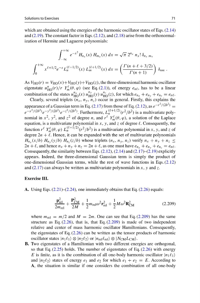
and (2.19). The constant factor in Eqs. (2.12), and (2.18) arise from the orthonormalization of Hermite and Laguerre polynomials:
+∞
−∞
e
−x 2
H n x (x) H m x (x) dx =
√
π 2
n x n x ! δ n x m x
+∞
0
x
+1/2 e
−x L
((+1/2)
n
(x) L
((+1/2)
m
(x) dx =
Γ (n + + 3/2)
Γ (n + 1)
δ nm .
As V HO (r) = V HO (x)+V HO (y)+V HO (z), the three-dimensional harmonic oscillator
eigenstate u n
HO (r)/r Y
m (θ, ϕ) (see Eq. (2.1)), of energy e nn , has to be a linear
combination of the states u
n x
HO (x) u
n y
HO (y) u
n z
HO (z), for which e n x + e n y + e n z = e nn .
Clearly, several triplets (n x , n y , n z ) occur in general. Firstly, this explains the
appearance of a Gaussian term in Eq. (2.17) from those of Eq. (2.12), as e −r 2 /(2b 2 ) =
e −x 2 /(2b 2 ) e −y 2 /(2b 2 ) e −z 2 /(2b 2 ) . Furthermore, L
((+1/2)
n
(r 2 /b 2 ) is a multivariate polynomial in x 2 , y 2 , and z 2 of degree n, and r Y
m (θ, ϕ), a solution of the Laplace
equation, is a multivariate polynomial in x, y, and z of degree . Consequently, the
function r Y
m (θ, ϕ) L
((+1/2)
n
(r 2 /b 2 ) is a multivariate polynomial in x, y, and z of
degree 2n + . Hence, it can be expanded with the set of multivariate polynomials
H n x (x/b) H n y (y/b) H n z (z/b) whose triplets (n x , n y , n z ) verify n x + n y + n z ≤
2n + , and hence n x + n y + n z = 2n + , as one must have e n x + e n y + e n z = e nn .
Consequently, the similarity between Eqs. (2.12), (2.14) and (2.17)–(2.19) explicitly
appears. Indeed, the three-dimensional Gaussian term is simply the product of
one-dimensional Gaussian terms, while the rest of wave functions in Eqs. (2.12)
and (2.17) can always be written as multivariate polynomials in x, y and z.
Exercise III.
A. Using Eqs. (2.21)–(2.24), one immediately obtains that Eq. (2.26) equals:
p 2
rel
2m rel
+
P 2
CM
2M
+
1
2
m rel ω
2 r
2
rel +
1
2
Mω
2 R
2
CM
(2.209)
where m rel = m/2 and M = 2m. One can see that Eq. (2.209) has the same
structure as Eq. (2.26), that is, that Eq. (2.209) is made of two independent
relative and center of mass harmonic oscillator Hamiltonians. Consequently,
the eigenstates of Eq. (2.26) can be written as the tensor products of harmonic
oscillator states |n 1 1 ⊗ |n 2 2 or |n rel rel ⊗ |N CM L CM
B. Two eigenstates of a Hamiltonian with two different energies are orthogonal,
so that Eq. (2.25) holds. The number of eigenstates of Eq. (2.26) with energy
E is finite, as it is the combination of all one-body harmonic oscillator |n 1 1
and |n 2 2 states of energy e 1 and e 2 for which e 1 + e 2 = E. According to
A, the situation is similar if one considers the combination of all one-body
71
which are obtained using the energies of the harmonic oscillator states of Eqs. (2.14)
and (2.19). The constant factor in Eqs. (2.12), and (2.18) arise from the orthonormalization of Hermite and Laguerre polynomials:
+∞
−∞
e
−x 2
H n x (x) H m x (x) dx =
√
π 2
n x n x ! δ n x m x
+∞
0
x
+1/2 e
−x L
((+1/2)
n
(x) L
((+1/2)
m
(x) dx =
Γ (n + + 3/2)
Γ (n + 1)
δ nm .
As V HO (r) = V HO (x)+V HO (y)+V HO (z), the three-dimensional harmonic oscillator
eigenstate u n
HO (r)/r Y
m (θ, ϕ) (see Eq. (2.1)), of energy e nn , has to be a linear
combination of the states u
n x
HO (x) u
n y
HO (y) u
n z
HO (z), for which e n x + e n y + e n z = e nn .
Clearly, several triplets (n x , n y , n z ) occur in general. Firstly, this explains the
appearance of a Gaussian term in Eq. (2.17) from those of Eq. (2.12), as e −r 2 /(2b 2 ) =
e −x 2 /(2b 2 ) e −y 2 /(2b 2 ) e −z 2 /(2b 2 ) . Furthermore, L
((+1/2)
n
(r 2 /b 2 ) is a multivariate polynomial in x 2 , y 2 , and z 2 of degree n, and r Y
m (θ, ϕ), a solution of the Laplace
equation, is a multivariate polynomial in x, y, and z of degree . Consequently, the
function r Y
m (θ, ϕ) L
((+1/2)
n
(r 2 /b 2 ) is a multivariate polynomial in x, y, and z of
degree 2n + . Hence, it can be expanded with the set of multivariate polynomials
H n x (x/b) H n y (y/b) H n z (z/b) whose triplets (n x , n y , n z ) verify n x + n y + n z ≤
2n + , and hence n x + n y + n z = 2n + , as one must have e n x + e n y + e n z = e nn .
Consequently, the similarity between Eqs. (2.12), (2.14) and (2.17)–(2.19) explicitly
appears. Indeed, the three-dimensional Gaussian term is simply the product of
one-dimensional Gaussian terms, while the rest of wave functions in Eqs. (2.12)
and (2.17) can always be written as multivariate polynomials in x, y and z.
Exercise III.
A. Using Eqs. (2.21)–(2.24), one immediately obtains that Eq. (2.26) equals:
p 2
rel
2m rel
+
P 2
CM
2M
+
1
2
m rel ω
2 r
2
rel +
1
2
Mω
2 R
2
CM
(2.209)
where m rel = m/2 and M = 2m. One can see that Eq. (2.209) has the same
structure as Eq. (2.26), that is, that Eq. (2.209) is made of two independent
relative and center of mass harmonic oscillator Hamiltonians. Consequently,
the eigenstates of Eq. (2.26) can be written as the tensor products of harmonic
oscillator states |n 1 1 ⊗ |n 2 2 or |n rel rel ⊗ |N CM L CM
B. Two eigenstates of a Hamiltonian with two different energies are orthogonal,
so that Eq. (2.25) holds. The number of eigenstates of Eq. (2.26) with energy
E is finite, as it is the combination of all one-body harmonic oscillator |n 1 1
and |n 2 2 states of energy e 1 and e 2 for which e 1 + e 2 = E. According to
A, the situation is similar if one considers the combination of all one-body