

2.6 Analytical Properties of the Wave Functions
61
-0.8
-0.6
-0.4
-0.2
0
0.2
0.4
0.6
0.8
0
5
10
15
20
25
30
u(r)
r(fm)
u
a
(r)
Im[u res (r)]
Re[u res (r)]
u
b
(r)
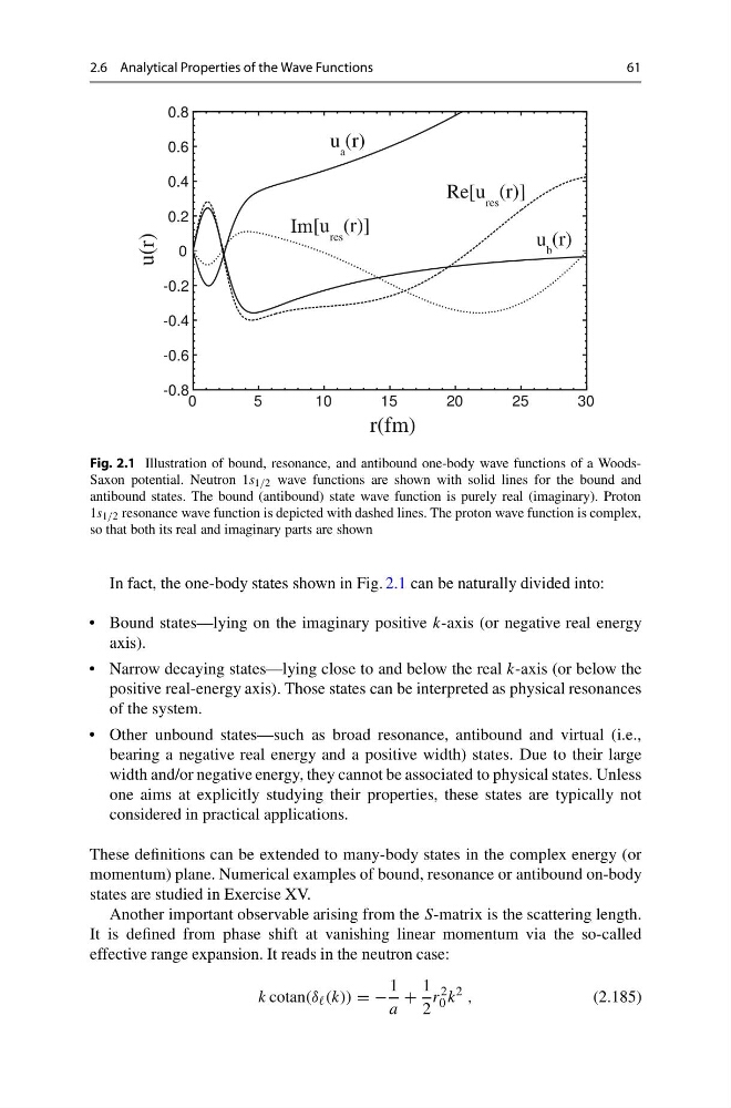
Fig. 2.1 Illustration of bound, resonance, and antibound one-body wave functions of a WoodsSaxon potential. Neutron 1s 1/2 wave functions are shown with solid lines for the bound and
antibound states. The bound (antibound) state wave function is purely real (imaginary). Proton
1s 1/2 resonance wave function is depicted with dashed lines. The proton wave function is complex,
so that both its real and imaginary parts are shown
In fact, the one-body states shown in Fig. 2.1 can be naturally divided into:
• Bound states—lying on the imaginary positive k-axis (or negative real energy
axis).
• Narrow decaying states—lying close to and below the real k-axis (or below the
positive real-energy axis). Those states can be interpreted as physical resonances
of the system.
• Other unbound states—such as broad resonance, antibound and virtual (i.e.,
bearing a negative real energy and a positive width) states. Due to their large
width and/or negative energy, they cannot be associated to physical states. Unless
one aims at explicitly studying their properties, these states are typically not
considered in practical applications.
These definitions can be extended to many-body states in the complex energy (or
momentum) plane. Numerical examples of bound, resonance or antibound on-body
states are studied in Exercise XV.
Another important observable arising from the S-matrix is the scattering length.
It is defined from phase shift at vanishing linear momentum via the so-called
effective range expansion. It reads in the neutron case:
k cotan(δ (k)) = −
1
a
+
1
2
r
2
0 k
2 ,
(2.185)
61
-0.8
-0.6
-0.4
-0.2
0
0.2
0.4
0.6
0.8
0
5
10
15
20
25
30
u(r)
r(fm)
u
a
(r)
Im[u res (r)]
Re[u res (r)]
u
b
(r)
Fig. 2.1 Illustration of bound, resonance, and antibound one-body wave functions of a WoodsSaxon potential. Neutron 1s 1/2 wave functions are shown with solid lines for the bound and
antibound states. The bound (antibound) state wave function is purely real (imaginary). Proton
1s 1/2 resonance wave function is depicted with dashed lines. The proton wave function is complex,
so that both its real and imaginary parts are shown
In fact, the one-body states shown in Fig. 2.1 can be naturally divided into:
• Bound states—lying on the imaginary positive k-axis (or negative real energy
axis).
• Narrow decaying states—lying close to and below the real k-axis (or below the
positive real-energy axis). Those states can be interpreted as physical resonances
of the system.
• Other unbound states—such as broad resonance, antibound and virtual (i.e.,
bearing a negative real energy and a positive width) states. Due to their large
width and/or negative energy, they cannot be associated to physical states. Unless
one aims at explicitly studying their properties, these states are typically not
considered in practical applications.
These definitions can be extended to many-body states in the complex energy (or
momentum) plane. Numerical examples of bound, resonance or antibound on-body
states are studied in Exercise XV.
Another important observable arising from the S-matrix is the scattering length.
It is defined from phase shift at vanishing linear momentum via the so-called
effective range expansion. It reads in the neutron case:
k cotan(δ (k)) = −
1
a
+
1
2
r
2
0 k
2 ,
(2.185)