

2.5 Basic Properties of Bound States
45
u(0, r) is equal to the number of bound states. Hence, the number of bound states is
finite and equal to the number of zeros of the u(0, r).
If v c < 0, the Hamiltonian models a hydrogenoid system, and one can show that
it has an infinite number of bound states. By continuity of u(k, r) in k = 0 for r
fixed (see Exercise XII) and from Eq. (2.59), there exists κ > 0 so that u(k, r) has n
nodes for n > 0. Hence, one can then generate a bound state u n−1 (r) of n − 1 nodes
by pushing the last node of an unbound u(k, r) state to r → +∞. This proves that
one has an infinity of bound states, which accumulate in k = 0.
2.5.2 Virial Theorem
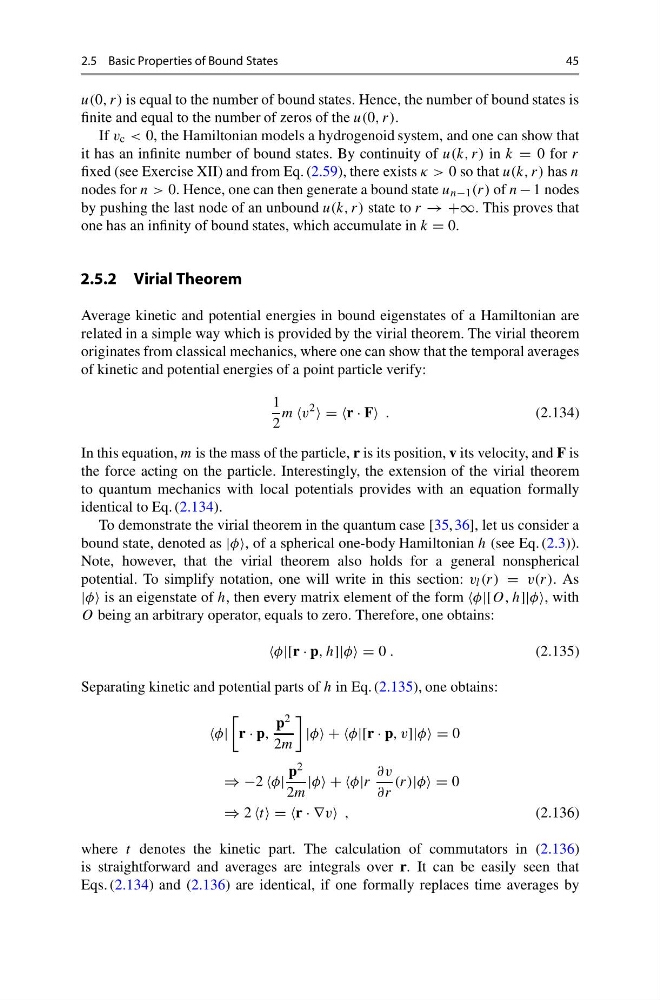
Average kinetic and potential energies in bound eigenstates of a Hamiltonian are
related in a simple way which is provided by the virial theorem. The virial theorem
originates from classical mechanics, where one can show that the temporal averages
of kinetic and potential energies of a point particle verify:
1
2
m
2
= =r · F .
(2.134)
In this equation, m is the mass of the particle, r is its position, v its velocity, and F is
the force acting on the particle. Interestingly, the extension of the virial theorem
to quantum mechanics with local potentials provides with an equation formally
identical to Eq. (2.134).
To demonstrate the virial theorem in the quantum case [35, 36], let us consider a
bound state, denoted as |φ, of a spherical one-body Hamiltonian h (see Eq. (2.3)).
Note, however, that the virial theorem also holds for a general nonspherical
potential. To simplify notation, one will write in this section: v l (r) = v(r). As
|φ is an eigenstate of h, then every matrix element of the form h]|φ, with
O being an arbitrary operator, equals to zero. Therefore, one obtains:
· p, h]|φ = 0 .
(2.135)
Separating kinetic and potential parts of h in Eq. (2.135), one obtains:
r · p,
p 2
2m
|φ + +φ|[r · p, v]|φ = 0
⇒ −2
p 2
2m
|φ + +φ|r
∂v
∂r
(r)|φ = 0
⇒ 2 = =r · ∇v ,
(2.136)
where t denotes the kinetic part. The calculation of commutators in (2.136)
is straightforward and averages are integrals over r. It can be easily seen that
Eqs. (2.134) and (2.136) are identical, if one formally replaces time averages by
45
u(0, r) is equal to the number of bound states. Hence, the number of bound states is
finite and equal to the number of zeros of the u(0, r).
If v c < 0, the Hamiltonian models a hydrogenoid system, and one can show that
it has an infinite number of bound states. By continuity of u(k, r) in k = 0 for r
fixed (see Exercise XII) and from Eq. (2.59), there exists κ > 0 so that u(k, r) has n
nodes for n > 0. Hence, one can then generate a bound state u n−1 (r) of n − 1 nodes
by pushing the last node of an unbound u(k, r) state to r → +∞. This proves that
one has an infinity of bound states, which accumulate in k = 0.
2.5.2 Virial Theorem
Average kinetic and potential energies in bound eigenstates of a Hamiltonian are
related in a simple way which is provided by the virial theorem. The virial theorem
originates from classical mechanics, where one can show that the temporal averages
of kinetic and potential energies of a point particle verify:
1
2
m
2
= =r · F .
(2.134)
In this equation, m is the mass of the particle, r is its position, v its velocity, and F is
the force acting on the particle. Interestingly, the extension of the virial theorem
to quantum mechanics with local potentials provides with an equation formally
identical to Eq. (2.134).
To demonstrate the virial theorem in the quantum case [35, 36], let us consider a
bound state, denoted as |φ, of a spherical one-body Hamiltonian h (see Eq. (2.3)).
Note, however, that the virial theorem also holds for a general nonspherical
potential. To simplify notation, one will write in this section: v l (r) = v(r). As
|φ is an eigenstate of h, then every matrix element of the form h]|φ, with
O being an arbitrary operator, equals to zero. Therefore, one obtains:
· p, h]|φ = 0 .
(2.135)
Separating kinetic and potential parts of h in Eq. (2.135), one obtains:
r · p,
p 2
2m
|φ + +φ|[r · p, v]|φ = 0
⇒ −2
p 2
2m
|φ + +φ|r
∂v
∂r
(r)|φ = 0
⇒ 2 = =r · ∇v ,
(2.136)
where t denotes the kinetic part. The calculation of commutators in (2.136)
is straightforward and averages are integrals over r. It can be easily seen that
Eqs. (2.134) and (2.136) are identical, if one formally replaces time averages by