

2.4 Pöschl-Teller-Ginocchio Potential
37
¯
ν =
ν +
1
2
2
− ¯
β 2
Λ 2 (1 − a) − 1
(2.104)
C
+
=
Γ (( +
3
2 )Γ (− ¯
β)
Γ (μ + )Γ (μ − )
, C
−
=
Γ (( +
3
2 )Γ ( ¯
β)
Γ (ν + )Γ (ν − )
(2.105)
f =
1 − y 2
1 − y 2 + Λ 2 y 2 , g =
Λ 2 y 2
1 − y 2 + Λ 2 y 2
(2.106)
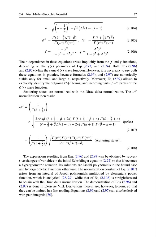
The r-dependence in these equations arises implicitly from the f and g functions,
depending on the y(r) parameter of Eqs. (2.73) and (2.74). Both Eqs. (2.96)
and (2.97) define the same φ(r) wave function. However, it is necessary to use both
these equations in practice, because formulas (2.96), and (2.97) are numerically
stable only for small and large r, respectively. Moreover, Eq. (2.97) allows to
explicitly identify the outgoing (“+” terms) and incoming parts (“−” terms) of the
φ(r) wave function.
Scattering states are normalized with the Dirac delta normalization. The N
normalization then reads:
N =
1
Γ (( +
3
2 )
×
2Λ 2 s ¯
β (( +
3
2 + ¯
β + 2n) Γ (( +
3
2 + ¯
β + n) Γ (( +
3
2 + n)
(( +
3
2 + ¯
βΛ 2 (1 − a) + 2n) Γ (n + 1) Γ ( ¯
β + n + 1)
(poles)
(2.107)
=
1
Γ (( +
3
2 )
Γ (ν + )Γ (ν − )Γ (μ + )Γ (μ − )
2π Γ ( ¯
β)Γ (− ¯
β)
(scattering states) .
(2.108)
The expressions resulting from Eqs. (2.96) and (2.97) can be obtained by successive changes of variables in the initial Schrödinger equation (2.72) so that it becomes
a hypergeometric equation. Its solutions are Jacobi polynomials in the bound case
and hypergeometric functions otherwise. The normalization constant of Eq. (2.107)
arises from an integral of Jacobi polynomials multiplied by elementary power
function, which is analytical [28, 29], while that of Eq. (2.108) is straightforward
to obtain with the Dirac delta normalization. The demonstration of Eqs. (2.96) and
(2.97) is done in Exercise VIII. Derivations therein are, however, tedious, so that
they can be omitted in a first reading. Equations (2.96) and (2.97) can also be derived
with path integrals [30].
37
¯
ν =
ν +
1
2
2
− ¯
β 2
Λ 2 (1 − a) − 1
(2.104)
C
+
=
Γ (( +
3
2 )Γ (− ¯
β)
Γ (μ + )Γ (μ − )
, C
−
=
Γ (( +
3
2 )Γ ( ¯
β)
Γ (ν + )Γ (ν − )
(2.105)
f =
1 − y 2
1 − y 2 + Λ 2 y 2 , g =
Λ 2 y 2
1 − y 2 + Λ 2 y 2
(2.106)
The r-dependence in these equations arises implicitly from the f and g functions,
depending on the y(r) parameter of Eqs. (2.73) and (2.74). Both Eqs. (2.96)
and (2.97) define the same φ(r) wave function. However, it is necessary to use both
these equations in practice, because formulas (2.96), and (2.97) are numerically
stable only for small and large r, respectively. Moreover, Eq. (2.97) allows to
explicitly identify the outgoing (“+” terms) and incoming parts (“−” terms) of the
φ(r) wave function.
Scattering states are normalized with the Dirac delta normalization. The N
normalization then reads:
N =
1
Γ (( +
3
2 )
×
2Λ 2 s ¯
β (( +
3
2 + ¯
β + 2n) Γ (( +
3
2 + ¯
β + n) Γ (( +
3
2 + n)
(( +
3
2 + ¯
βΛ 2 (1 − a) + 2n) Γ (n + 1) Γ ( ¯
β + n + 1)
(poles)
(2.107)
=
1
Γ (( +
3
2 )
Γ (ν + )Γ (ν − )Γ (μ + )Γ (μ − )
2π Γ ( ¯
β)Γ (− ¯
β)
(scattering states) .
(2.108)
The expressions resulting from Eqs. (2.96) and (2.97) can be obtained by successive changes of variables in the initial Schrödinger equation (2.72) so that it becomes
a hypergeometric equation. Its solutions are Jacobi polynomials in the bound case
and hypergeometric functions otherwise. The normalization constant of Eq. (2.107)
arises from an integral of Jacobi polynomials multiplied by elementary power
function, which is analytical [28, 29], while that of Eq. (2.108) is straightforward
to obtain with the Dirac delta normalization. The demonstration of Eqs. (2.96) and
(2.97) is done in Exercise VIII. Derivations therein are, however, tedious, so that
they can be omitted in a first reading. Equations (2.96) and (2.97) can also be derived
with path integrals [30].