

38
2 The Discrete Spectrum and the Continuum
Exercise VIII
One will show that the analytical formulas of Eqs. (2.96) and (2.97) are indeed
solving Eq. (2.72).
Show that the wave function defined in Eq. (2.96) is a solution of Eq. (2.72)
by a direct insertion of Eq. (2.96) in Eq. (2.72).
Deduce Eq. (2.97) from Eq. (2.96) using the following standard property of
the hypergeometric function:
2 F 1 (a, b, c; z) =
Γ (c)Γ (c − a − b)
Γ (c − a)Γ (c − b)
2 F 1 (a, b, a + b − c + 1; 1 − z)
+(1 − z)
c−a−b Γ (c)Γ (a + b − c)
Γ (a)Γ (b)
(2.109)
× 2 F 1 (c − a, c − b, c − a − b + 1; 1 − z)
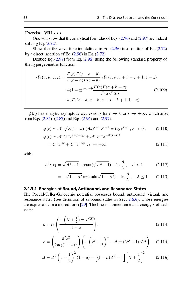
φ(r) has analytic asymptotic expressions for r → 0 or r → +∞, which arise
from Eqs. (2.85)–(2.87) and Eqs. (2.96) and (2.97):
φ(r) ∼ N
Λ(1 − a) (Λs)
r
+1
= C 0 r
+1 , r → 0 ,
(2.110)
φ(r) ∼ N C
+ e
ik(r−r 1 )
+ N C
− e
−ik(r−r 1 )
= C
+ e
ikr
+ C
− e
−ikr , r → +∞
(2.111)
with:
Λ
2 s r 1 =
Λ 2 − 1 arctan(
Λ 2 − 1) − ln
Λ
2
, Λ > 1
(2.112)
= −
1 − Λ 2 arctanh(
1 − Λ 2 ) − ln
Λ
2
, Λ ≤ 1
(2.113)
2.4.3.1 Energies of Bound, Antibound, and Resonance States
The Pöschl-Teller-Ginocchio potential possesses bound, antibound, virtual, and
resonance states (see definition of unbound states in Sect. 2.6.6), whose energies
are expressible in a closed form [29]. The linear momentum k and energy e of each
state:
k = is
⎛
⎝
−
N +
1
2
±
√
Δ
1 − a
⎞
⎠ ,
(2.114)
e =
¯
h
2 s 2
2m 0 (1 − a) 2
−
N +
1
2
2
− Δ ± (2N + 1)
√
Δ
(2.115)
Δ = Λ
2
ν +
1
2
2
(1 − a) −
(1 − a)Λ
2
− 1
N +
1
2
2
(2.116)
2 The Discrete Spectrum and the Continuum
Exercise VIII
One will show that the analytical formulas of Eqs. (2.96) and (2.97) are indeed
solving Eq. (2.72).
Show that the wave function defined in Eq. (2.96) is a solution of Eq. (2.72)
by a direct insertion of Eq. (2.96) in Eq. (2.72).
Deduce Eq. (2.97) from Eq. (2.96) using the following standard property of
the hypergeometric function:
2 F 1 (a, b, c; z) =
Γ (c)Γ (c − a − b)
Γ (c − a)Γ (c − b)
2 F 1 (a, b, a + b − c + 1; 1 − z)
+(1 − z)
c−a−b Γ (c)Γ (a + b − c)
Γ (a)Γ (b)
(2.109)
× 2 F 1 (c − a, c − b, c − a − b + 1; 1 − z)
φ(r) has analytic asymptotic expressions for r → 0 or r → +∞, which arise
from Eqs. (2.85)–(2.87) and Eqs. (2.96) and (2.97):
φ(r) ∼ N
Λ(1 − a) (Λs)
r
+1
= C 0 r
+1 , r → 0 ,
(2.110)
φ(r) ∼ N C
+ e
ik(r−r 1 )
+ N C
− e
−ik(r−r 1 )
= C
+ e
ikr
+ C
− e
−ikr , r → +∞
(2.111)
with:
Λ
2 s r 1 =
Λ 2 − 1 arctan(
Λ 2 − 1) − ln
Λ
2
, Λ > 1
(2.112)
= −
1 − Λ 2 arctanh(
1 − Λ 2 ) − ln
Λ
2
, Λ ≤ 1
(2.113)
2.4.3.1 Energies of Bound, Antibound, and Resonance States
The Pöschl-Teller-Ginocchio potential possesses bound, antibound, virtual, and
resonance states (see definition of unbound states in Sect. 2.6.6), whose energies
are expressible in a closed form [29]. The linear momentum k and energy e of each
state:
k = is
⎛
⎝
−
N +
1
2
±
√
Δ
1 − a
⎞
⎠ ,
(2.114)
e =
¯
h
2 s 2
2m 0 (1 − a) 2
−
N +
1
2
2
− Δ ± (2N + 1)
√
Δ
(2.115)
Δ = Λ
2
ν +
1
2
2
(1 − a) −
(1 − a)Λ
2
− 1
N +
1
2
2
(2.116)