9.2 Generalization to Many-Nucleon Projectiles
427
method becomes not applicable when the number of nucleons increases, as the use
of Jacobi coordinates becomes cumbersome in this situation [35, 36]. In practice,
this method might be useful for projectiles bearing two or three nucleons only.
9.2.4 Berggren Basis Expansion of Center-of-Mass States
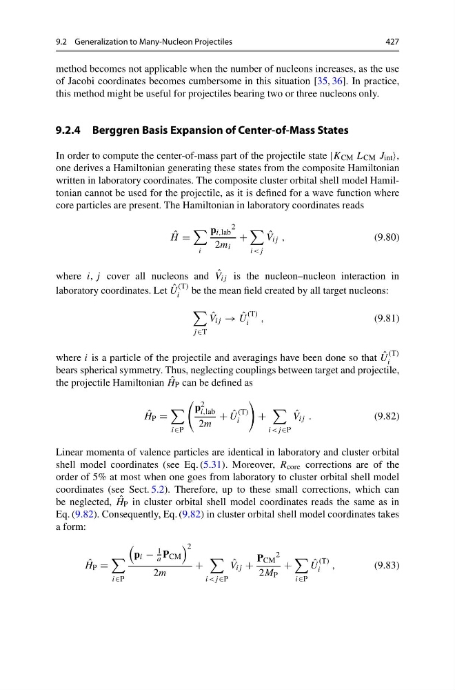
In order to compute the center-of-mass part of the projectile state |K CM L CM J int
one derives a Hamiltonian generating these states from the composite Hamiltonian
written in laboratory coordinates. The composite cluster orbital shell model Hamiltonian cannot be used for the projectile, as it is defined for a wave function where
core particles are present. The Hamiltonian in laboratory coordinates reads
ˆ
H =
i
p i,lab
2
2m i
+
i ˆ
V ij ,
(9.80)
where i, j cover all nucleons and ˆ
V ij is the nucleon–nucleon interaction in
laboratory coordinates. Let ˆ
U
(T)
i
be the mean field created by all target nucleons:
j ∈T
ˆ
V ij → ˆ
U
(T)
i
,
(9.81)
where i is a particle of the projectile and averagings have been done so that ˆ
U
(T)
i
bears spherical symmetry. Thus, neglecting couplings between target and projectile,
the projectile Hamiltonian ˆ
H P can be defined as
ˆ
H P =
i∈P
p 2
i,lab
2m
+ ˆ
U
(T)
i
+
i ˆ
V ij .
(9.82)
Linear momenta of valence particles are identical in laboratory and cluster orbital
shell model coordinates (see Eq. (5.31). Moreover, R core corrections are of the
order of 5% at most when one goes from laboratory to cluster orbital shell model
coordinates (see Sect. 5.2). Therefore, up to these small corrections, which can
be neglected, ˆ
H P in cluster orbital shell model coordinates reads the same as in
Eq. (9.82). Consequently, Eq. (9.82) in cluster orbital shell model coordinates takes
a form:
ˆ
H P =
i∈P
p i −
1
a P CM
2
2m
+
i ˆ
V ij +
P CM
2
2M P
+
i∈P
ˆ
U
(T)
i ,
(9.83)