

258
6 Physical Applications of the Gamow Shell Model
bound but the many-body state is unbound, the corresponding contour was defined
by the points k peak = (0.25, −0.24) fm −1 , k mid = (0.5, 0.0) fm −1 , and k max =
(2.0, 0.0) fm −1 to generate a many-body configuration space which can describe an
unbound many-body state. In all cases, the three segments were discretized with at
least ten Gauss-Legendre points. The remaining higher- partial waves, and proton
partial waves in neutron-rich nuclei, which play no role in the asymptotic region
for the considered nuclei, were described using a harmonic oscillator basis. For that
matter, and to reduce the size of the model space, the sdf partial waves for protons
and df partial waves for neutrons were described by a harmonic oscillator basis with
11 shells (n HO
max = 10). In this mixed basis, the natural orbitals were generated as
discussed in Sect. 5.3 what allowed to have up to the four particles in the scattering
continuum.
The two-body interaction was optimized to the experimental binding energies
of the ground states and a few selected excited states of the helium, lithium, and
beryllium isotopes. The binding energies with respect to 4 He span a large energy
range, from approximately −30 MeV to +2 MeV, and different types of states are
involved: bound states, resonances, and halo states, as for the ground state of 6 He.
The optimization provided a χ 2 minimum with a precision 2 /N dof ∼ 10 −4
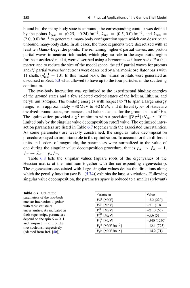
limited only by the singular value decomposition cutoff value. The optimized interaction parameters are listed in Table 6.7 together with the associated uncertainties.
As some parameters are weakly constrained, the singular value decomposition
procedure played an important role in the optimization. To account for their different
units and orders of magnitude, the parameters were normalized to the value of
one during the singular value decomposition procedure, that is p α → ˜
p α = 1,
J iα → ˜
J iα = p α J iα .
Table 6.8 lists the singular values (square roots of the eigenvalues of the
Hessian matrix at the minimum together with the corresponding eigenvectors).
The eigenvectors associated with large singular values define the directions along
which the penalty function (see Eq. (5.74)) exhibits the largest variations. Following
singular value decomposition, the parameter space is reduced to a smaller (relevant)
Table 6.7 Optimized
parameters of the two-body
nuclear interaction together
with their statistical
uncertainties. As indicated in
their superscript, parameters
depend on the spin S = 0, 1
and isospin T = 0, 1 of the
two nucleons, respectively
(adapted from Ref. [40])
Parameter
Value
V 11
C [MeV]
−3.2 (220)
V 10
C [MeV]
−5.1 (10)
V
00
C [MeV]
−21.3 (66)
V 01
C [MeV]
−5.6 (5)
V 11
LS [MeV]
−540 (1240)
V 11
T [MeV fm −2 ]
−12.1 (795)
V 10
T [MeV fm −2 ]
−14.2 (71)
6 Physical Applications of the Gamow Shell Model
bound but the many-body state is unbound, the corresponding contour was defined
by the points k peak = (0.25, −0.24) fm −1 , k mid = (0.5, 0.0) fm −1 , and k max =
(2.0, 0.0) fm −1 to generate a many-body configuration space which can describe an
unbound many-body state. In all cases, the three segments were discretized with at
least ten Gauss-Legendre points. The remaining higher- partial waves, and proton
partial waves in neutron-rich nuclei, which play no role in the asymptotic region
for the considered nuclei, were described using a harmonic oscillator basis. For that
matter, and to reduce the size of the model space, the sdf partial waves for protons
and df partial waves for neutrons were described by a harmonic oscillator basis with
11 shells (n HO
max = 10). In this mixed basis, the natural orbitals were generated as
discussed in Sect. 5.3 what allowed to have up to the four particles in the scattering
continuum.
The two-body interaction was optimized to the experimental binding energies
of the ground states and a few selected excited states of the helium, lithium, and
beryllium isotopes. The binding energies with respect to 4 He span a large energy
range, from approximately −30 MeV to +2 MeV, and different types of states are
involved: bound states, resonances, and halo states, as for the ground state of 6 He.
The optimization provided a χ 2 minimum with a precision 2 /N dof ∼ 10 −4
limited only by the singular value decomposition cutoff value. The optimized interaction parameters are listed in Table 6.7 together with the associated uncertainties.
As some parameters are weakly constrained, the singular value decomposition
procedure played an important role in the optimization. To account for their different
units and orders of magnitude, the parameters were normalized to the value of
one during the singular value decomposition procedure, that is p α → ˜
p α = 1,
J iα → ˜
J iα = p α J iα .
Table 6.8 lists the singular values (square roots of the eigenvalues of the
Hessian matrix at the minimum together with the corresponding eigenvectors).
The eigenvectors associated with large singular values define the directions along
which the penalty function (see Eq. (5.74)) exhibits the largest variations. Following
singular value decomposition, the parameter space is reduced to a smaller (relevant)
Table 6.7 Optimized
parameters of the two-body
nuclear interaction together
with their statistical
uncertainties. As indicated in
their superscript, parameters
depend on the spin S = 0, 1
and isospin T = 0, 1 of the
two nucleons, respectively
(adapted from Ref. [40])
Parameter
Value
V 11
C [MeV]
−3.2 (220)
V 10
C [MeV]
−5.1 (10)
V
00
C [MeV]
−21.3 (66)
V 01
C [MeV]
−5.6 (5)
V 11
LS [MeV]
−540 (1240)
V 11
T [MeV fm −2 ]
−12.1 (795)
V 10
T [MeV fm −2 ]
−14.2 (71)