

5.1 Mathematical Foundation of the Gamow Shell Model
189
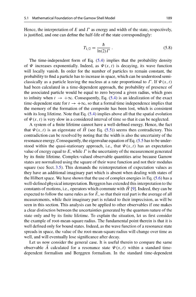
Hence, the interpretation of E and Γ as energy and width of the state, respectively,
is justified, and one can define the half-life of the state correspondingly:
T 1/2 =
¯
h
ln(2)Γ
.
(5.8)
The time-independent form of Eq. (5.4) implies that the probability density
of Ψ increases exponentially. Indeed, as Ψ (x, t) is decaying, its wave function
will locally vanish. In order for the number of particles to remain constant, the
probability to find a particle has to increase in space, which can be understood semiclassically as a particle leaving the nucleus at a rate proportional to Γ . If Ψ (x, t)
had been calculated in a time-dependent approach, the probability of presence of
the associated particle would be equal to zero beyond a given radius, which goes
to infinity when t → +∞. Consequently, Eq. (5.4) is an idealization of the exact
time-dependent state for t → +∞, so that a formal time independence implies that
the memory of the formation of the composite has been lost, which is consistent
with its long lifetime. Note that Eq. (5.4) implies above all that the spatial evolution
of Ψ (x, t) is very slow in a considered interval of time so that it can be neglected.
A system of a finite lifetime cannot have a well-defined energy. Hence, the fact
that Ψ (x, t) is an eigenstate of ˆ
H (see Eq. (5.5)) seems then contradictory. This
contradiction can be resolved by noting that the width is also the uncertainty of the
resonance energy. Consequently, the eigenvalue equation of Eq. (5.5 has to be understood within the quasi-stationary approach, i.e., that Ψ (x, t) has an expectation
value of energy equal to E, while Γ is the uncertainty of the measurement generated
by its finite lifetime. Complex-valued observable quantities arise because Gamow
states are normalized using the square of their wave function and not their modulus
square (see Sect. 3.5). This demands the reinterpretation of expectation values as
they have an additional imaginary part which is absent when dealing with states of
the Hilbert space. We have shown that the use of complex energies in Eq. (5.6) has a
well-defined physical interpretation. Berggren has extended this interpretation to the
constants of motions, i.e., operators which commute with ˆ
H [9]. Indeed, they can be
expected to follow the same rules as for ˜
E, so that their real part is the average of all
measurements, while their imaginary part is related to their imprecision, as will be
seen in this section. This analysis can be applied to other observables if one makes
a clear distinction between the uncertainties generated by the quantum nature of the
state only and by its finite lifetime. To explain the situation, let us first consider
the example of root-mean-square radius. The fundamental point therein is that it is
well defined only for bound states. Indeed, as the wave function of a resonance state
spreads in space, the value of the root-mean-square radius will change over time as
well, and will eventually lose significance after decay.
Let us now consider the general case. It is useful therein to compare the same
observable ˆ
A calculated for a resonance state Ψ (x, t) within a standard timedependent formalism and Berggren formalism. In the standard time-dependent
189
Hence, the interpretation of E and Γ as energy and width of the state, respectively,
is justified, and one can define the half-life of the state correspondingly:
T 1/2 =
¯
h
ln(2)Γ
.
(5.8)
The time-independent form of Eq. (5.4) implies that the probability density
of Ψ increases exponentially. Indeed, as Ψ (x, t) is decaying, its wave function
will locally vanish. In order for the number of particles to remain constant, the
probability to find a particle has to increase in space, which can be understood semiclassically as a particle leaving the nucleus at a rate proportional to Γ . If Ψ (x, t)
had been calculated in a time-dependent approach, the probability of presence of
the associated particle would be equal to zero beyond a given radius, which goes
to infinity when t → +∞. Consequently, Eq. (5.4) is an idealization of the exact
time-dependent state for t → +∞, so that a formal time independence implies that
the memory of the formation of the composite has been lost, which is consistent
with its long lifetime. Note that Eq. (5.4) implies above all that the spatial evolution
of Ψ (x, t) is very slow in a considered interval of time so that it can be neglected.
A system of a finite lifetime cannot have a well-defined energy. Hence, the fact
that Ψ (x, t) is an eigenstate of ˆ
H (see Eq. (5.5)) seems then contradictory. This
contradiction can be resolved by noting that the width is also the uncertainty of the
resonance energy. Consequently, the eigenvalue equation of Eq. (5.5 has to be understood within the quasi-stationary approach, i.e., that Ψ (x, t) has an expectation
value of energy equal to E, while Γ is the uncertainty of the measurement generated
by its finite lifetime. Complex-valued observable quantities arise because Gamow
states are normalized using the square of their wave function and not their modulus
square (see Sect. 3.5). This demands the reinterpretation of expectation values as
they have an additional imaginary part which is absent when dealing with states of
the Hilbert space. We have shown that the use of complex energies in Eq. (5.6) has a
well-defined physical interpretation. Berggren has extended this interpretation to the
constants of motions, i.e., operators which commute with ˆ
H [9]. Indeed, they can be
expected to follow the same rules as for ˜
E, so that their real part is the average of all
measurements, while their imaginary part is related to their imprecision, as will be
seen in this section. This analysis can be applied to other observables if one makes
a clear distinction between the uncertainties generated by the quantum nature of the
state only and by its finite lifetime. To explain the situation, let us first consider
the example of root-mean-square radius. The fundamental point therein is that it is
well defined only for bound states. Indeed, as the wave function of a resonance state
spreads in space, the value of the root-mean-square radius will change over time as
well, and will eventually lose significance after decay.
Let us now consider the general case. It is useful therein to compare the same
observable ˆ
A calculated for a resonance state Ψ (x, t) within a standard timedependent formalism and Berggren formalism. In the standard time-dependent