

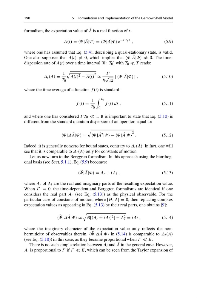
190
5 Formulation and Implementation of the Gamow Shell Model
formalism, the expectation value of ˆ
A is a real function of t:
A(t) = =Ψ | ˆ
A|Ψ = =Φ| ˆ
A|Φ e
−Γ t/¯ h ,
(5.9)
where one has assumed that Eq. (5.4), describing a quasi-stationary state, is valid.
One also supposes that A(t) = 0, which implies that ˆ
A|Φ = 0. The timedispersion rate of A(t) over a time interval [0 : T 0 ] with T 0 T reads:
Δ t (A) =
1
T 0
A(t) 2 − A(t)
2
Γ
¯
h
√
12
| |Φ| ˆ
A|Φ | ,
(5.10)
where the time average of a function f (t) is standard:
f (t) =
1
T 0
T 0
0
f (t) dt ,
(5.11)
and where one has considered Γ T 0 1. It is important to state that Eq. (5.10) is
different from the standard quantum dispersion of an operator, equal to:
|Δ ˆ
A|Ψ =
| ˆ
A 2 |Ψ − −Ψ | ˆ
A|Ψ
2 .
(5.12)
Indeed, it is generally nonzero for bound states, contrary to Δ t (A). In fact, one will
see that it is comparable to Δ t (A) only for constants of motion.
Let us now turn to the Berggren formalism. In this approach using the biorthogonal basis (see Sect. 5.1.1), Eq. (5.9) becomes:
Φ| ˆ
A|Φ = A r + iA i ,
(5.13)
where A r of A i are the real and imaginary parts of the resulting expectation value.
When Γ = 0, the time-dependent and Berggren formalisms are identical if one
considers the real part A r (see Eq. (5.13)) as the physical observable. For the
particular case of constants of motion, where [H, A] = 0, then replacing complex
expectation values as appearing in Eq. (5.13) by their real parts, one obtains [9]:
Φ|Δ ˆ
A|Φ
[(A r + iA i ) 2 ] − A 2
r = iA i ,
(5.14)
where the imaginary character of the expectation value only reflects the nonhermiticity of observables therein.
Φ|Δ ˆ
A|Φ in (5.14) is comparable to Δ t (A)
(see Eq. (5.10)) in this case, as they become proportional when Γ E.
There is no such simple relation between A i and ˆ
A in the general case. However,
A i is proportional to Γ if Γ E, which can be seen from the Taylor expansion of
5 Formulation and Implementation of the Gamow Shell Model
formalism, the expectation value of ˆ
A is a real function of t:
A(t) = =Ψ | ˆ
A|Ψ = =Φ| ˆ
A|Φ e
−Γ t/¯ h ,
(5.9)
where one has assumed that Eq. (5.4), describing a quasi-stationary state, is valid.
One also supposes that A(t) = 0, which implies that ˆ
A|Φ = 0. The timedispersion rate of A(t) over a time interval [0 : T 0 ] with T 0 T reads:
Δ t (A) =
1
T 0
A(t) 2 − A(t)
2
Γ
¯
h
√
12
| |Φ| ˆ
A|Φ | ,
(5.10)
where the time average of a function f (t) is standard:
f (t) =
1
T 0
T 0
0
f (t) dt ,
(5.11)
and where one has considered Γ T 0 1. It is important to state that Eq. (5.10) is
different from the standard quantum dispersion of an operator, equal to:
|Δ ˆ
A|Ψ =
| ˆ
A 2 |Ψ − −Ψ | ˆ
A|Ψ
2 .
(5.12)
Indeed, it is generally nonzero for bound states, contrary to Δ t (A). In fact, one will
see that it is comparable to Δ t (A) only for constants of motion.
Let us now turn to the Berggren formalism. In this approach using the biorthogonal basis (see Sect. 5.1.1), Eq. (5.9) becomes:
Φ| ˆ
A|Φ = A r + iA i ,
(5.13)
where A r of A i are the real and imaginary parts of the resulting expectation value.
When Γ = 0, the time-dependent and Berggren formalisms are identical if one
considers the real part A r (see Eq. (5.13)) as the physical observable. For the
particular case of constants of motion, where [H, A] = 0, then replacing complex
expectation values as appearing in Eq. (5.13) by their real parts, one obtains [9]:
Φ|Δ ˆ
A|Φ
[(A r + iA i ) 2 ] − A 2
r = iA i ,
(5.14)
where the imaginary character of the expectation value only reflects the nonhermiticity of observables therein.
Φ|Δ ˆ
A|Φ in (5.14) is comparable to Δ t (A)
(see Eq. (5.10)) in this case, as they become proportional when Γ E.
There is no such simple relation between A i and ˆ
A in the general case. However,
A i is proportional to Γ if Γ E, which can be seen from the Taylor expansion of