

3.7 Numerical Implementation of the Berggren Completeness Relation
125
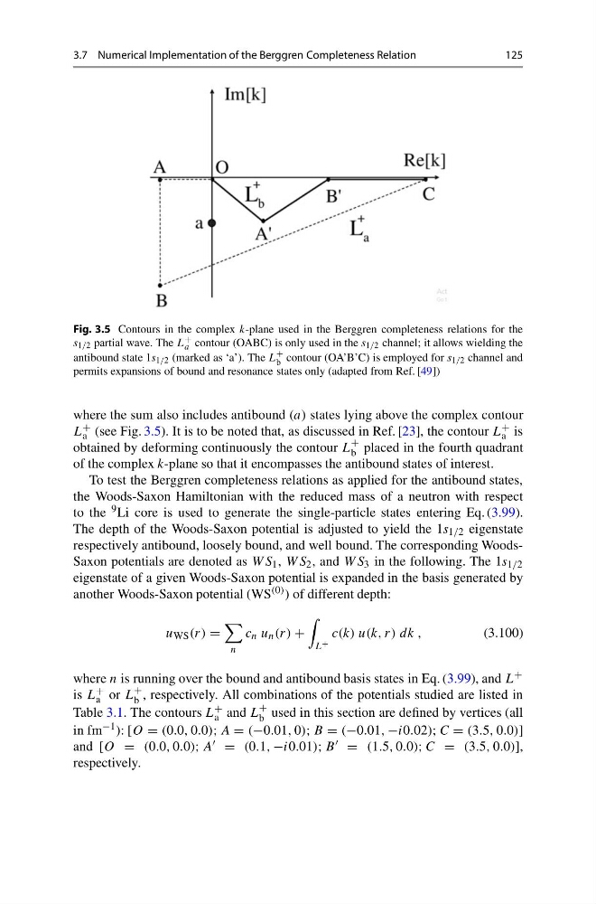
Fig. 3.5 Contours in the complex k-plane used in the Berggren completeness relations for the
s 1/2 partial wave. The L +
a contour (OABC) is only used in the s 1/2 channel; it allows wielding the
antibound state 1s 1/2 (marked as ‘a’). The L
+
b contour (OA’B’C) is employed for s 1/2 channel and
permits expansions of bound and resonance states only (adapted from Ref. [49])
where the sum also includes antibound (a) states lying above the complex contour
L +
a (see Fig. 3.5). It is to be noted that, as discussed in Ref. [23], the contour L +
a is
obtained by deforming continuously the contour L
+
b placed in the fourth quadrant
of the complex k-plane so that it encompasses the antibound states of interest.
To test the Berggren completeness relations as applied for the antibound states,
the Woods-Saxon Hamiltonian with the reduced mass of a neutron with respect
to the 9 Li core is used to generate the single-particle states entering Eq. (3.99).
The depth of the Woods-Saxon potential is adjusted to yield the 1s 1/2 eigenstate
respectively antibound, loosely bound, and well bound. The corresponding WoodsSaxon potentials are denoted as W S 1 , W S 2 , and W S 3 in the following. The 1s 1/2
eigenstate of a given Woods-Saxon potential is expanded in the basis generated by
another Woods-Saxon potential (WS (0) ) of different depth:
u WS (r) =
n
c n u n (r) +
L +
c(k) u(k, r) dk ,
(3.100)
where n is running over the bound and antibound basis states in Eq. (3.99), and L +
is L +
a or L
+
b , respectively. All combinations of the potentials studied are listed in
Table 3.1. The contours L +
a and L
+
b used in this section are defined by vertices (all
in fm −1 ): [O = (0.0, 0.0); A = (−0.01, 0); B = (−0.01, −i0.02); C = (3.5, 0.0)]
and [O = (0.0, 0.0); A = (0.1, −i0.01); B = (1.5, 0.0); C = (3.5, 0.0)],
respectively.
125
Fig. 3.5 Contours in the complex k-plane used in the Berggren completeness relations for the
s 1/2 partial wave. The L +
a contour (OABC) is only used in the s 1/2 channel; it allows wielding the
antibound state 1s 1/2 (marked as ‘a’). The L
+
b contour (OA’B’C) is employed for s 1/2 channel and
permits expansions of bound and resonance states only (adapted from Ref. [49])
where the sum also includes antibound (a) states lying above the complex contour
L +
a (see Fig. 3.5). It is to be noted that, as discussed in Ref. [23], the contour L +
a is
obtained by deforming continuously the contour L
+
b placed in the fourth quadrant
of the complex k-plane so that it encompasses the antibound states of interest.
To test the Berggren completeness relations as applied for the antibound states,
the Woods-Saxon Hamiltonian with the reduced mass of a neutron with respect
to the 9 Li core is used to generate the single-particle states entering Eq. (3.99).
The depth of the Woods-Saxon potential is adjusted to yield the 1s 1/2 eigenstate
respectively antibound, loosely bound, and well bound. The corresponding WoodsSaxon potentials are denoted as W S 1 , W S 2 , and W S 3 in the following. The 1s 1/2
eigenstate of a given Woods-Saxon potential is expanded in the basis generated by
another Woods-Saxon potential (WS (0) ) of different depth:
u WS (r) =
n
c n u n (r) +
L +
c(k) u(k, r) dk ,
(3.100)
where n is running over the bound and antibound basis states in Eq. (3.99), and L +
is L +
a or L
+
b , respectively. All combinations of the potentials studied are listed in
Table 3.1. The contours L +
a and L
+
b used in this section are defined by vertices (all
in fm −1 ): [O = (0.0, 0.0); A = (−0.01, 0); B = (−0.01, −i0.02); C = (3.5, 0.0)]
and [O = (0.0, 0.0); A = (0.1, −i0.01); B = (1.5, 0.0); C = (3.5, 0.0)],
respectively.