

126
3 Berggren Basis and Completeness Relations
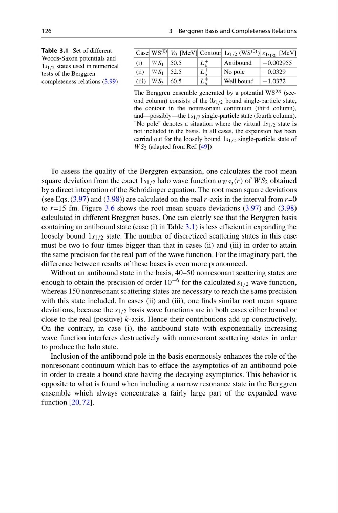
Table 3.1 Set of different
Woods-Saxon potentials and
1s 1/2 states used in numerical
tests of the Berggren
completeness relations (3.99)
Case WS (0) V 0 [MeV] Contour 1s 1/2 (WS (0) ) ε 1s 1/2 [MeV]
(i) W S 1 50.5
L +
a
Antibound
−0.002955
(ii) W S 1 52.5
L
+
b
No pole
−0.0329
(iii) W S 3 60.5
L
+
b
Well bound −1.0372
The Berggren ensemble generated by a potential WS (0) (second column) consists of the 0s 1/2 bound single-particle state,
the contour in the nonresonant continuum (third column),
and—possibly—the 1s 1/2 single-particle state (fourth column).
"No pole" denotes a situation where the virtual 1s 1/2 state is
not included in the basis. In all cases, the expansion has been
carried out for the loosely bound 1s 1/2 single-particle state of
W S 2 (adapted from Ref. [49])
To assess the quality of the Berggren expansion, one calculates the root mean
square deviation from the exact 1s 1/2 halo wave function u W S 2 (r) of W S 2 obtained
by a direct integration of the Schrödinger equation. The root mean square deviations
(see Eqs. (3.97) and (3.98)) are calculated on the real r-axis in the interval from r=0
to r=15 fm. Figure 3.6 shows the root mean square deviations (3.97) and (3.98)
calculated in different Breggren bases. One can clearly see that the Berggren basis
containing an antibound state (case (i) in Table 3.1) is less efficient in expanding the
loosely bound 1s 1/2 state. The number of discretized scattering states in this case
must be two to four times bigger than that in cases (ii) and (iii) in order to attain
the same precision for the real part of the wave function. For the imaginary part, the
difference between results of these bases is even more pronounced.
Without an antibound state in the basis, 40–50 nonresonant scattering states are
enough to obtain the precision of order 10 −6 for the calculated s 1/2 wave function,
whereas 150 nonresonant scattering states are necessary to reach the same precision
with this state included. In cases (ii) and (iii), one finds similar root mean square
deviations, because the s 1/2 basis wave functions are in both cases either bound or
close to the real (positive) k-axis. Hence their contributions add up constructively.
On the contrary, in case (i), the antibound state with exponentially increasing
wave function interferes destructively with nonresonant scattering states in order
to produce the halo state.
Inclusion of the antibound pole in the basis enormously enhances the role of the
nonresonant continuum which has to efface the asymptotics of an antibound pole
in order to create a bound state having the decaying asymptotics. This behavior is
opposite to what is found when including a narrow resonance state in the Berggren
ensemble which always concentrates a fairly large part of the expanded wave
function [20, 72].
3 Berggren Basis and Completeness Relations
Table 3.1 Set of different
Woods-Saxon potentials and
1s 1/2 states used in numerical
tests of the Berggren
completeness relations (3.99)
Case WS (0) V 0 [MeV] Contour 1s 1/2 (WS (0) ) ε 1s 1/2 [MeV]
(i) W S 1 50.5
L +
a
Antibound
−0.002955
(ii) W S 1 52.5
L
+
b
No pole
−0.0329
(iii) W S 3 60.5
L
+
b
Well bound −1.0372
The Berggren ensemble generated by a potential WS (0) (second column) consists of the 0s 1/2 bound single-particle state,
the contour in the nonresonant continuum (third column),
and—possibly—the 1s 1/2 single-particle state (fourth column).
"No pole" denotes a situation where the virtual 1s 1/2 state is
not included in the basis. In all cases, the expansion has been
carried out for the loosely bound 1s 1/2 single-particle state of
W S 2 (adapted from Ref. [49])
To assess the quality of the Berggren expansion, one calculates the root mean
square deviation from the exact 1s 1/2 halo wave function u W S 2 (r) of W S 2 obtained
by a direct integration of the Schrödinger equation. The root mean square deviations
(see Eqs. (3.97) and (3.98)) are calculated on the real r-axis in the interval from r=0
to r=15 fm. Figure 3.6 shows the root mean square deviations (3.97) and (3.98)
calculated in different Breggren bases. One can clearly see that the Berggren basis
containing an antibound state (case (i) in Table 3.1) is less efficient in expanding the
loosely bound 1s 1/2 state. The number of discretized scattering states in this case
must be two to four times bigger than that in cases (ii) and (iii) in order to attain
the same precision for the real part of the wave function. For the imaginary part, the
difference between results of these bases is even more pronounced.
Without an antibound state in the basis, 40–50 nonresonant scattering states are
enough to obtain the precision of order 10 −6 for the calculated s 1/2 wave function,
whereas 150 nonresonant scattering states are necessary to reach the same precision
with this state included. In cases (ii) and (iii), one finds similar root mean square
deviations, because the s 1/2 basis wave functions are in both cases either bound or
close to the real (positive) k-axis. Hence their contributions add up constructively.
On the contrary, in case (i), the antibound state with exponentially increasing
wave function interferes destructively with nonresonant scattering states in order
to produce the halo state.
Inclusion of the antibound pole in the basis enormously enhances the role of the
nonresonant continuum which has to efface the asymptotics of an antibound pole
in order to create a bound state having the decaying asymptotics. This behavior is
opposite to what is found when including a narrow resonance state in the Berggren
ensemble which always concentrates a fairly large part of the expanded wave
function [20, 72].