

3.7 Numerical Implementation of the Berggren Completeness Relation
113
of bound and resonance states is one to two orders of magnitude smaller than the
number of discretized basis scattering states. The use of a truncated Berggren basis,
where one removes all scattering states, is called the pole approximation, as one
leaves only S-matrix poles in the Berggren basis (3.82).
3.7.1 Completeness Relations Involving Proton States
In this section, we shall discuss numerical examples of the Berggren completeness
relation in the one-proton case, as it was theoretically considered in Sect. 3.5.
Contrary to the previous sections, the efficiency of the Berggren completeness
relation from a computational point of view will be demonstrated. Indeed, while
Eq. (3.82) directly leads to a matrix of finite dimension to be diagonalized, one still
has to demonstrate that it is of practical use, that is, that the method described in
Sect. 3.7 leads to a fast and stable numerical algorithm.
For this, one will consider the diagonalization of a Woods-Saxon potential with
the Berggren basis generated by another Woods-Saxon potential. Indeed, one can
then directly check the precision of diagonalized eigenstates by comparing them
to the quasi-exact wave functions obtained from a direct integration of Eq. (2.2).
Dealing with the resonances is difficult in the proton case due to the singular
character of the scattering functions in the complex k-plane (see Sect. 2.3).
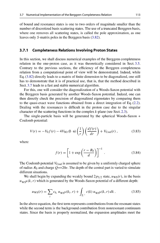
The single-particle basis will be generated by the spherical Woods-Saxon +
Coulomb potential:
V (r) = −V 0 f (r) − 4V SO (l · s)
1
r
df (r)
dr
+ V Coul (r) ,
(3.83)
where
f (r) =
1 + exp
r − R 0
d
−1
.
(3.84)
The Coulomb potential V Coul is assumed to be given by a uniformly charged sphere
of radius R 0 and charge Q=+20e. The depth of the central part is varied to simulate
different situations.
We shall begin by expanding the weakly bound 2p 3/2 state, u WS (r), in the basis
u WS B (k, r) which is generated by the Woods-Saxon potential of a different depth:
u WS (r) =
i
c k i u WS B (k i , r) +
L +
c(k) u WS B (k, r) dk .
(3.85)
In the above equation, the first term represents contributions from the resonant states
while the second term is the background contribution from nonresonant continuum
states. Since the basis is properly normalized, the expansion amplitudes meet the
113
of bound and resonance states is one to two orders of magnitude smaller than the
number of discretized basis scattering states. The use of a truncated Berggren basis,
where one removes all scattering states, is called the pole approximation, as one
leaves only S-matrix poles in the Berggren basis (3.82).
3.7.1 Completeness Relations Involving Proton States
In this section, we shall discuss numerical examples of the Berggren completeness
relation in the one-proton case, as it was theoretically considered in Sect. 3.5.
Contrary to the previous sections, the efficiency of the Berggren completeness
relation from a computational point of view will be demonstrated. Indeed, while
Eq. (3.82) directly leads to a matrix of finite dimension to be diagonalized, one still
has to demonstrate that it is of practical use, that is, that the method described in
Sect. 3.7 leads to a fast and stable numerical algorithm.
For this, one will consider the diagonalization of a Woods-Saxon potential with
the Berggren basis generated by another Woods-Saxon potential. Indeed, one can
then directly check the precision of diagonalized eigenstates by comparing them
to the quasi-exact wave functions obtained from a direct integration of Eq. (2.2).
Dealing with the resonances is difficult in the proton case due to the singular
character of the scattering functions in the complex k-plane (see Sect. 2.3).
The single-particle basis will be generated by the spherical Woods-Saxon +
Coulomb potential:
V (r) = −V 0 f (r) − 4V SO (l · s)
1
r
df (r)
dr
+ V Coul (r) ,
(3.83)
where
f (r) =
1 + exp
r − R 0
d
−1
.
(3.84)
The Coulomb potential V Coul is assumed to be given by a uniformly charged sphere
of radius R 0 and charge Q=+20e. The depth of the central part is varied to simulate
different situations.
We shall begin by expanding the weakly bound 2p 3/2 state, u WS (r), in the basis
u WS B (k, r) which is generated by the Woods-Saxon potential of a different depth:
u WS (r) =
i
c k i u WS B (k i , r) +
L +
c(k) u WS B (k, r) dk .
(3.85)
In the above equation, the first term represents contributions from the resonant states
while the second term is the background contribution from nonresonant continuum
states. Since the basis is properly normalized, the expansion amplitudes meet the