

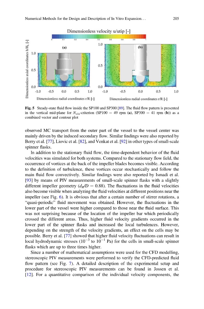
observed MC transport from the outer part of the vessel to the vessel center was
mainly driven by the induced secondary flow. Similar findings were also reported by
Berry et al. [77], Liovic et al. [82], and Venkat et al. [92] in other types of small-scale
spinner flasks.
In addition to the stationary fluid flow, the time-dependent behavior of the fluid
velocities was simulated for both systems. Compared to the stationary flow field, the
occurrence of vortices at the back of the impeller blades becomes visible. According
to the definition of turbulence, these vortices occur stochastically and follow the
main fluid flow convectively. Similar findings were also reported by Ismadi et al.
[93] by means of PIV measurements of small-scale spinner flasks with a slightly
different impeller geometry (d R /D ¼ 0.88). The fluctuations in the fluid velocities
also become visible when analyzing the fluid velocities at different positions near the
impeller (see Fig. 6). It is obvious that after a certain number of stirrer rotations, a
“quasi-periodic” fluid movement was obtained. However, the fluctuations in the
lower part of the vessel were higher compared to those near the fluid surface. This
was not surprising because of the location of the impeller bar which periodically
crossed the different areas. Thus, higher fluid velocity gradients occurred in the
lower part of the spinner flasks and increased the local turbulences. However,
depending on the strength of the velocity gradients, an effect on the cells may be
possible. Berry et al. [77] showed that higher fluid velocity fluctuations can result in
local hydrodynamic stresses (10
À3 to 10
À1 Pa) for the cells in small-scale spinner
flasks which are up to three times higher.
Since a number of mathematical assumptions were used for the CFD modelling,
stereoscopic PIV measurements were performed to verify the CFD-predicted fluid
flow pattern (see Fig. 7). A detailed description of the experimental setup and
procedure for stereoscopic PIV measurements can be found in Jossen et al.
[12]. For a quantitative comparison of the individual velocity components, the
Fig. 5 Steady-state fluid flow inside the SP100 and SP300 [89]. The fluid flow pattern is presented
in the vertical mid-plane for N s1u -criterion (SP100 ¼ 49 rpm (a), SP300 ¼ 41 rpm (b)) as a
combined vector and contour plot
Numerical Methods for the Design and Description of In Vitro Expansion. . .
205
mainly driven by the induced secondary flow. Similar findings were also reported by
Berry et al. [77], Liovic et al. [82], and Venkat et al. [92] in other types of small-scale
spinner flasks.
In addition to the stationary fluid flow, the time-dependent behavior of the fluid
velocities was simulated for both systems. Compared to the stationary flow field, the
occurrence of vortices at the back of the impeller blades becomes visible. According
to the definition of turbulence, these vortices occur stochastically and follow the
main fluid flow convectively. Similar findings were also reported by Ismadi et al.
[93] by means of PIV measurements of small-scale spinner flasks with a slightly
different impeller geometry (d R /D ¼ 0.88). The fluctuations in the fluid velocities
also become visible when analyzing the fluid velocities at different positions near the
impeller (see Fig. 6). It is obvious that after a certain number of stirrer rotations, a
“quasi-periodic” fluid movement was obtained. However, the fluctuations in the
lower part of the vessel were higher compared to those near the fluid surface. This
was not surprising because of the location of the impeller bar which periodically
crossed the different areas. Thus, higher fluid velocity gradients occurred in the
lower part of the spinner flasks and increased the local turbulences. However,
depending on the strength of the velocity gradients, an effect on the cells may be
possible. Berry et al. [77] showed that higher fluid velocity fluctuations can result in
local hydrodynamic stresses (10
À3 to 10
À1 Pa) for the cells in small-scale spinner
flasks which are up to three times higher.
Since a number of mathematical assumptions were used for the CFD modelling,
stereoscopic PIV measurements were performed to verify the CFD-predicted fluid
flow pattern (see Fig. 7). A detailed description of the experimental setup and
procedure for stereoscopic PIV measurements can be found in Jossen et al.
[12]. For a quantitative comparison of the individual velocity components, the
Fig. 5 Steady-state fluid flow inside the SP100 and SP300 [89]. The fluid flow pattern is presented
in the vertical mid-plane for N s1u -criterion (SP100 ¼ 49 rpm (a), SP300 ¼ 41 rpm (b)) as a
combined vector and contour plot
Numerical Methods for the Design and Description of In Vitro Expansion. . .
205