

x f , k
½ ¼ x k
½ þ K k
½ z k
½ À Cx k
½
À
Á
ð5Þ
P f , k
½ ¼ P k
½ 1 À K k
½ C
À
Á 2 þ K
2 R
ð6Þ
K k
½ ¼ P k
½ C
T R þ CP k
½ C
T
À
Á À1
ð7Þ
The measurement prediction error, reflects the discrepancy between the true
measurements z [k] and the predicted measurements Cx [k] . The difference of both is
multiplied by the so called Kalman gain and used to update the estimated state
variables. Therefore the filtered state variables x f, [k] are obtained. In the similar
manner, the filtered estimation error covariance P f, [k] is obtained. K [k] is chosen to
minimizes the estimated error covariance
dP f
dK
¼ 0
ð8Þ
The measurement error variance must be compared with the estimation error
variance to see how the filter is acting. For this purpose, a very rough treatment is
necessary:
If R ( CP [k] C
T then K % C
À1 and x f, [k] % C
À1 z [k] ; so the filtered is almost
determined by the measured.
If R ) CP [k] C
T then x f, [k] % x [k] ; the filtered value is almost the estimated one and
no influence of the measurement will be obtained.
With the filtered values as initial condition the simulation of the process as well as
the estimation error covariance’s can be carried out until the next measurement is
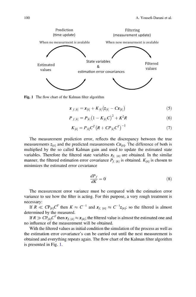
obtained and everything repeats again. The flow chart of the Kalman filter algorithm
is presented in Fig. 1.
Prediction
(Ɵme update)
Filtering
(measurement update)
State variables
&
esƟmaƟon error covariances
Filtered
values
Estimated
values
When new measurment is avalable
When no measurment is avalable
Fig. 1 The flow chart of the Kalman filter algorithm
100
A. Yousefi-Darani et al.
½ ¼ x k
½ þ K k
½ z k
½ À Cx k
½
À
Á
ð5Þ
P f , k
½ ¼ P k
½ 1 À K k
½ C
À
Á 2 þ K
2 R
ð6Þ
K k
½ ¼ P k
½ C
T R þ CP k
½ C
T
À
Á À1
ð7Þ
The measurement prediction error, reflects the discrepancy between the true
measurements z [k] and the predicted measurements Cx [k] . The difference of both is
multiplied by the so called Kalman gain and used to update the estimated state
variables. Therefore the filtered state variables x f, [k] are obtained. In the similar
manner, the filtered estimation error covariance P f, [k] is obtained. K [k] is chosen to
minimizes the estimated error covariance
dP f
dK
¼ 0
ð8Þ
The measurement error variance must be compared with the estimation error
variance to see how the filter is acting. For this purpose, a very rough treatment is
necessary:
If R ( CP [k] C
T then K % C
À1 and x f, [k] % C
À1 z [k] ; so the filtered is almost
determined by the measured.
If R ) CP [k] C
T then x f, [k] % x [k] ; the filtered value is almost the estimated one and
no influence of the measurement will be obtained.
With the filtered values as initial condition the simulation of the process as well as
the estimation error covariance’s can be carried out until the next measurement is
obtained and everything repeats again. The flow chart of the Kalman filter algorithm
is presented in Fig. 1.
Prediction
(Ɵme update)
Filtering
(measurement update)
State variables
&
esƟmaƟon error covariances
Filtered
values
Estimated
values
When new measurment is avalable
When no measurment is avalable
Fig. 1 The flow chart of the Kalman filter algorithm
100
A. Yousefi-Darani et al.