

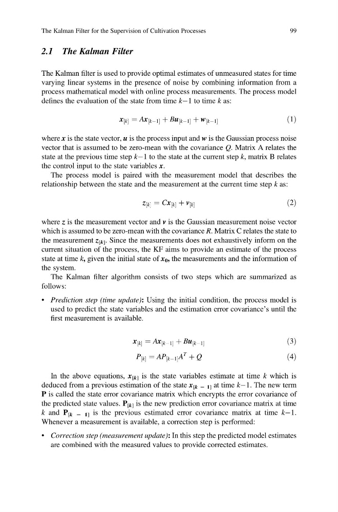
2.1 The Kalman Filter
The Kalman filter is used to provide optimal estimates of unmeasured states for time
varying linear systems in the presence of noise by combining information from a
process mathematical model with online process measurements. The process model
defines the evaluation of the state from time kÀ1 to time k as:
x k
½ ¼ Ax kÀ1
½
þ Bu kÀ1
½
þ w kÀ1
½
ð1Þ
where x is the state vector, u is the process input and w is the Gaussian process noise
vector that is assumed to be zero-mean with the covariance Q. Matrix A relates the
state at the previous time step kÀ1 to the state at the current step k, matrix B relates
the control input to the state variables x.
The process model is paired with the measurement model that describes the
relationship between the state and the measurement at the current time step k as:
z k
½ ¼ Cx k
½ þ v k
½
ð2Þ
where z is the measurement vector and v is the Gaussian measurement noise vector
which is assumed to be zero-mean with the covariance R. Matrix C relates the state to
the measurement z [k] . Since the measurements does not exhaustively inform on the
current situation of the process, the KF aims to provide an estimate of the process
state at time k, given the initial state of x 0 , the measurements and the information of
the system.
The Kalman filter algorithm consists of two steps which are summarized as
follows:
• Prediction step (time update): Using the initial condition, the process model is
used to predict the state variables and the estimation error covariance’s until the
first measurement is available.
x k
½ ¼ Ax kÀ1
½
þ Bu kÀ1
½
ð3Þ
P k
½ ¼ AP kÀ1
½
A
T
þ Q
ð4Þ
In the above equations, x [k] is the state variables estimate at time k which is
deduced from a previous estimation of the state x [k 2 1] at time kÀ1. The new term
P is called the state error covariance matrix which encrypts the error covariance of
the predicted state values. P [k] is the new prediction error covariance matrix at time
k and P [k 2 1] is the previous estimated error covariance matrix at time kÀ1.
Whenever a measurement is available, a correction step is performed:
• Correction step (measurement update): In this step the predicted model estimates
are combined with the measured values to provide corrected estimates.
The Kalman Filter for the Supervision of Cultivation Processes
99
The Kalman filter is used to provide optimal estimates of unmeasured states for time
varying linear systems in the presence of noise by combining information from a
process mathematical model with online process measurements. The process model
defines the evaluation of the state from time kÀ1 to time k as:
x k
½ ¼ Ax kÀ1
½
þ Bu kÀ1
½
þ w kÀ1
½
ð1Þ
where x is the state vector, u is the process input and w is the Gaussian process noise
vector that is assumed to be zero-mean with the covariance Q. Matrix A relates the
state at the previous time step kÀ1 to the state at the current step k, matrix B relates
the control input to the state variables x.
The process model is paired with the measurement model that describes the
relationship between the state and the measurement at the current time step k as:
z k
½ ¼ Cx k
½ þ v k
½
ð2Þ
where z is the measurement vector and v is the Gaussian measurement noise vector
which is assumed to be zero-mean with the covariance R. Matrix C relates the state to
the measurement z [k] . Since the measurements does not exhaustively inform on the
current situation of the process, the KF aims to provide an estimate of the process
state at time k, given the initial state of x 0 , the measurements and the information of
the system.
The Kalman filter algorithm consists of two steps which are summarized as
follows:
• Prediction step (time update): Using the initial condition, the process model is
used to predict the state variables and the estimation error covariance’s until the
first measurement is available.
x k
½ ¼ Ax kÀ1
½
þ Bu kÀ1
½
ð3Þ
P k
½ ¼ AP kÀ1
½
A
T
þ Q
ð4Þ
In the above equations, x [k] is the state variables estimate at time k which is
deduced from a previous estimation of the state x [k 2 1] at time kÀ1. The new term
P is called the state error covariance matrix which encrypts the error covariance of
the predicted state values. P [k] is the new prediction error covariance matrix at time
k and P [k 2 1] is the previous estimated error covariance matrix at time kÀ1.
Whenever a measurement is available, a correction step is performed:
• Correction step (measurement update): In this step the predicted model estimates
are combined with the measured values to provide corrected estimates.
The Kalman Filter for the Supervision of Cultivation Processes
99