

2.1 Bivectors and Electromagnetic Fields
25
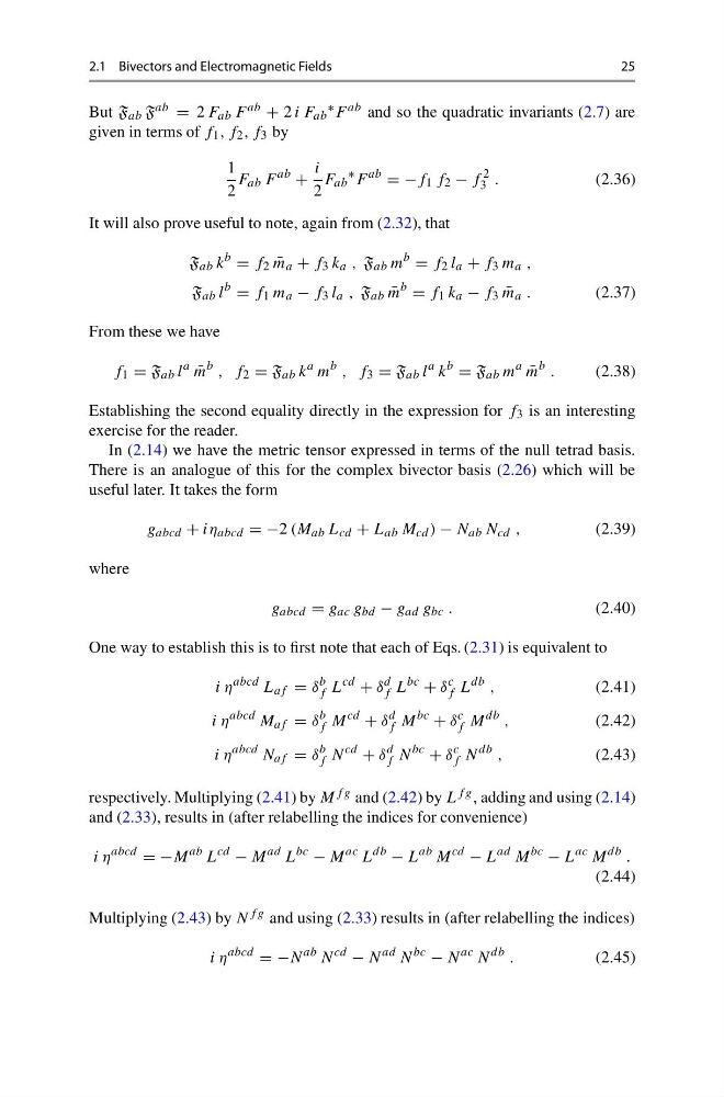
But F ab F ab = 2 F ab F ab + 2 i F ab
∗ F ab and so the quadratic invariants (2.7) are
given in terms of f 1 , f 2 , f 3 by
1
2
F ab F
ab
+
i
2
F ab
∗ F
ab
= −f 1 f 2 − f
2
3 .
(2.36)
It will also prove useful to note, again from (2.32), that
F ab k
b
= f 2 ¯
m a + f 3 k a , F ab m
b
= f 2 l a + f 3 m a ,
F ab l
b
= f 1 m a − f 3 l a , F ab ¯
m
b
= f 1 k a − f 3 ¯
m a .
(2.37)
From these we have
f 1 = F ab l
a
¯
m
b , f 2 = F ab k
a m
b , f 3 = F ab l
a k
b
= F ab m
a
¯
m
b .
(2.38)
Establishing the second equality directly in the expression for f 3 is an interesting
exercise for the reader.
In (2.14) we have the metric tensor expressed in terms of the null tetrad basis.
There is an analogue of this for the complex bivector basis (2.26) which will be
useful later. It takes the form
g abcd + iη abcd = −2 (M ab L cd + L ab M cd ) − N ab N cd ,
(2.39)
where
g abcd = g ac g bd − g ad g bc .
(2.40)
One way to establish this is to first note that each of Eqs. (2.31) is equivalent to
i η
abcd L af = δ
b
f L
cd
+ δ
d
f L
bc
+ δ
c
f L
db ,
(2.41)
i η
abcd M af = δ
b
f M
cd
+ δ
d
f M
bc
+ δ
c
f M
db ,
(2.42)
i η
abcd N af = δ
b
f N
cd
+ δ
d
f N
bc
+ δ
c
f N
db ,
(2.43)
respectively. Multiplying (2.41) by M fg and (2.42) by L fg , adding and using (2.14)
and (2.33), results in (after relabelling the indices for convenience)
i η
abcd
= −M
ab L
cd
− M
ad L
bc
− M
ac L
db
− L
ab M
cd
− L
ad M
bc
− L
ac M
db .
(2.44)
Multiplying (2.43) by N fg and using (2.33) results in (after relabelling the indices)
i η
abcd
= −N
ab N
cd
− N
ad N
bc
− N
ac N
db .
(2.45)
25
But F ab F ab = 2 F ab F ab + 2 i F ab
∗ F ab and so the quadratic invariants (2.7) are
given in terms of f 1 , f 2 , f 3 by
1
2
F ab F
ab
+
i
2
F ab
∗ F
ab
= −f 1 f 2 − f
2
3 .
(2.36)
It will also prove useful to note, again from (2.32), that
F ab k
b
= f 2 ¯
m a + f 3 k a , F ab m
b
= f 2 l a + f 3 m a ,
F ab l
b
= f 1 m a − f 3 l a , F ab ¯
m
b
= f 1 k a − f 3 ¯
m a .
(2.37)
From these we have
f 1 = F ab l
a
¯
m
b , f 2 = F ab k
a m
b , f 3 = F ab l
a k
b
= F ab m
a
¯
m
b .
(2.38)
Establishing the second equality directly in the expression for f 3 is an interesting
exercise for the reader.
In (2.14) we have the metric tensor expressed in terms of the null tetrad basis.
There is an analogue of this for the complex bivector basis (2.26) which will be
useful later. It takes the form
g abcd + iη abcd = −2 (M ab L cd + L ab M cd ) − N ab N cd ,
(2.39)
where
g abcd = g ac g bd − g ad g bc .
(2.40)
One way to establish this is to first note that each of Eqs. (2.31) is equivalent to
i η
abcd L af = δ
b
f L
cd
+ δ
d
f L
bc
+ δ
c
f L
db ,
(2.41)
i η
abcd M af = δ
b
f M
cd
+ δ
d
f M
bc
+ δ
c
f M
db ,
(2.42)
i η
abcd N af = δ
b
f N
cd
+ δ
d
f N
bc
+ δ
c
f N
db ,
(2.43)
respectively. Multiplying (2.41) by M fg and (2.42) by L fg , adding and using (2.14)
and (2.33), results in (after relabelling the indices for convenience)
i η
abcd
= −M
ab L
cd
− M
ad L
bc
− M
ac L
db
− L
ab M
cd
− L
ad M
bc
− L
ac M
db .
(2.44)
Multiplying (2.43) by N fg and using (2.33) results in (after relabelling the indices)
i η
abcd
= −N
ab N
cd
− N
ad N
bc
− N
ac N
db .
(2.45)