

2.1 Bivectors and Electromagnetic Fields
23
where the scalar V is real-valued and is given by
V = −i η
abcd
¯
m a m b l c k d = −i η abcd ¯
m
a m
b l
c k
d .
(2.22)
Hence it follows from (2.21) that (m a k b − m b k a ) is one of the basis complex
bivectors we seek provided we can demonstrate that we can choose V = −1. In
similar fashion the reader can verify that
∗ ( ¯
m
a l
b
− ¯
m
b l
a ) = i V ( ¯
m
a l
b
− ¯
m
b l
a ) .
(2.23)
Also
∗ ( ¯
m
a m
b
− ¯
m
b m
a ) = i V (k
a l
b
− k
b l
a ) and
∗ (k
a l
b
− k
b l
a ) = i V ( ¯
m
a m
b
− ¯
m
b m
a ) ,
(2.24)
from which we have
∗ ( ¯
m
a m
b
− ¯
m
b m
a
+k
a l
b
−k
b l
a ) = i V ( ¯
m
a m
b
− ¯
m
b m
a
+k
a l
b
−k
b l
a ) . (2.25)
Hence the three candidates for basis complex bivectors are
L ab = m a k b − m b k a = −L ba , M ab = ¯
m a l b − ¯
m b l a = −M ba ,
N ab = ¯
m a m b − ¯
m b m a + k a l b − k b l a = −N ba .
(2.26)
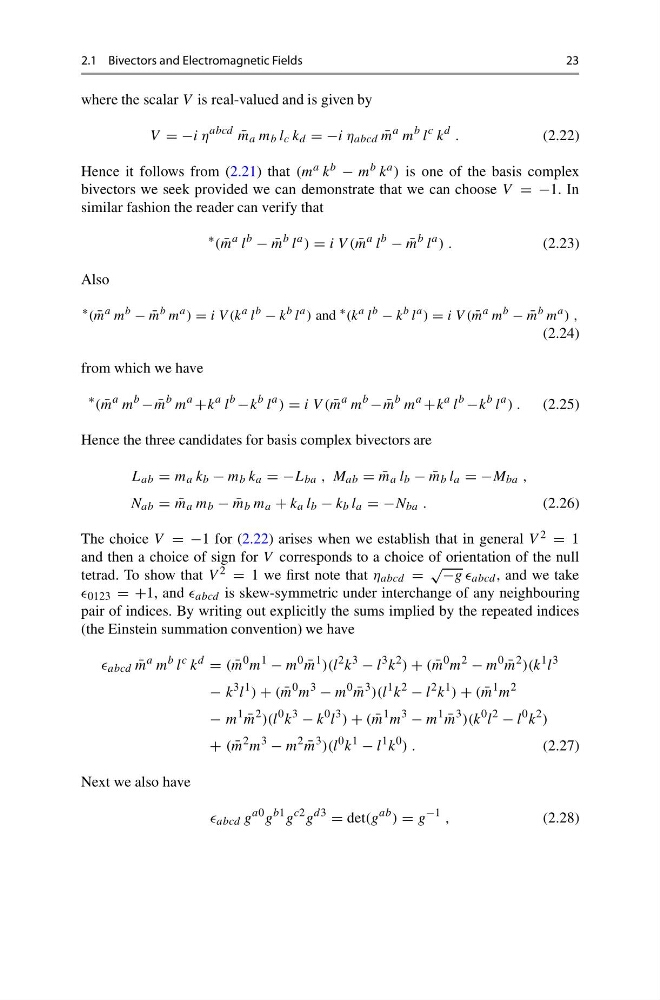
The choice V = −1 for (2.22) arises when we establish that in general V 2 = 1
and then a choice of sign for V corresponds to a choice of orientation of the null
tetrad. To show that V 2 = 1 we first note that η abcd =
√
−g g abcd , and we take
0123 = +1, and abcd is skew-symmetric under interchange of any neighbouring
pair of indices. By writing out explicitly the sums implied by the repeated indices
(the Einstein summation convention) we have
abcd ¯
m
a m
b l
c k
d
= ( ¯
m
0 m
1
− m
0
¯
m
1 )(l
2 k
3
− l
3 k
2 ) + ( ¯
m
0 m
2
− m
0
¯
m
2 )(k
1 l
3
− k
3 l
1 ) + ( ¯
m
0 m
3
− m
0
¯
m
3 )(l
1 k
2
− l
2 k
1 ) + ( ¯
m
1 m
2
− m
1
¯
m
2 )(l
0 k
3
− k
0 l
3 ) + ( ¯
m
1 m
3
− m
1
¯
m
3 )(k
0 l
2
− l
0 k
2 )
+ ( ¯
m
2 m
3
− m
2
¯
m
3 )(l
0 k
1
− l
1 k
0 ) .
(2.27)
Next we also have
abcd g
a0 g
b1 g
c2 g
d3
= det(g
ab ) = g
−1 ,
(2.28)
23
where the scalar V is real-valued and is given by
V = −i η
abcd
¯
m a m b l c k d = −i η abcd ¯
m
a m
b l
c k
d .
(2.22)
Hence it follows from (2.21) that (m a k b − m b k a ) is one of the basis complex
bivectors we seek provided we can demonstrate that we can choose V = −1. In
similar fashion the reader can verify that
∗ ( ¯
m
a l
b
− ¯
m
b l
a ) = i V ( ¯
m
a l
b
− ¯
m
b l
a ) .
(2.23)
Also
∗ ( ¯
m
a m
b
− ¯
m
b m
a ) = i V (k
a l
b
− k
b l
a ) and
∗ (k
a l
b
− k
b l
a ) = i V ( ¯
m
a m
b
− ¯
m
b m
a ) ,
(2.24)
from which we have
∗ ( ¯
m
a m
b
− ¯
m
b m
a
+k
a l
b
−k
b l
a ) = i V ( ¯
m
a m
b
− ¯
m
b m
a
+k
a l
b
−k
b l
a ) . (2.25)
Hence the three candidates for basis complex bivectors are
L ab = m a k b − m b k a = −L ba , M ab = ¯
m a l b − ¯
m b l a = −M ba ,
N ab = ¯
m a m b − ¯
m b m a + k a l b − k b l a = −N ba .
(2.26)
The choice V = −1 for (2.22) arises when we establish that in general V 2 = 1
and then a choice of sign for V corresponds to a choice of orientation of the null
tetrad. To show that V 2 = 1 we first note that η abcd =
√
−g g abcd , and we take
0123 = +1, and abcd is skew-symmetric under interchange of any neighbouring
pair of indices. By writing out explicitly the sums implied by the repeated indices
(the Einstein summation convention) we have
abcd ¯
m
a m
b l
c k
d
= ( ¯
m
0 m
1
− m
0
¯
m
1 )(l
2 k
3
− l
3 k
2 ) + ( ¯
m
0 m
2
− m
0
¯
m
2 )(k
1 l
3
− k
3 l
1 ) + ( ¯
m
0 m
3
− m
0
¯
m
3 )(l
1 k
2
− l
2 k
1 ) + ( ¯
m
1 m
2
− m
1
¯
m
2 )(l
0 k
3
− k
0 l
3 ) + ( ¯
m
1 m
3
− m
1
¯
m
3 )(k
0 l
2
− l
0 k
2 )
+ ( ¯
m
2 m
3
− m
2
¯
m
3 )(l
0 k
1
− l
1 k
0 ) .
(2.27)
Next we also have
abcd g
a0 g
b1 g
c2 g
d3
= det(g
ab ) = g
−1 ,
(2.28)