

8.4 EOMs of a Reissner–Nordström Particle
199
Now with C
1
(u) = 0 and (8.77) holding we have
K 1 = 6 e
2 V 1 .
(8.82)
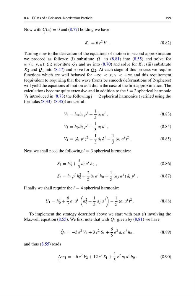
Turning now to the derivation of the equations of motion in second approximation
we proceed as follows: (i) substitute Q 1 in (8.81) into (8.55) and solve for
w 1 (x, y, u); (ii) substitute Q 1 and w 1 into (8.70) and solve for K 2 ; (iii) substitute
K 2 and Q 1 into (8.47) and solve for Q 2 . At each stage of this process we require
functions which are well behaved for −∞ < x, y < +∞ and this requirement
(equivalent to requiring that the wave fronts be smooth deformations of 2-spheres)
will yield the equations of motion as it did in the case of the first approximation. The
calculations become quite extensive and in addition to the l = 2 spherical harmonic
V 1 introduced in (8.73) the following l = 2 spherical harmonics (verified using the
formulas (8.33)–(8.35)) are useful:
V 2 = h 0 ˙
a i p
i
+
1
3
˙
a i a
i ,
(8.83)
V 3 = h 0 ¨
a i p
i
+
1
3
a i ¨
a
i ,
(8.84)
V 4 = ( ˙
a i p
i )
2
+
1
3
˙
a i ˙
a
i
−
1
3
(a i a
i )
2 .
(8.85)
Next we shall need the following l = 3 spherical harmonics:
S 1 = h
3
0 +
3
5
a i a
i h 0 ,
(8.86)
S 2 = ˙
a i p
i h
2
0 +
2
5
˙
a i a
i h 0 +
1
5
(a j a
j ) ˙
a i p
i .
(8.87)
Finally we shall require the l = 4 spherical harmonic:
U 1 = h
4
0 +
6
7
a i a
i
h
2
0 +
1
3
a j a
j
−
1
5
(a i a
i )
2 .
(8.88)
To implement the strategy described above we start with part (i) involving the
Maxwell equation (8.55). We first note that with Q 1 given by (8.81) we have
˙
Q 1 = −3 e
2 V 2 + 3 e
2 S 1 +
6
5
e
2 a i a
i h 0 ,
(8.89)
and thus (8.55) reads
0
w 1 = −6 e
2 V 2 + 12 e
2 S 1 +
4
5
e
2 a i a
i h 0 .
(8.90)
199
Now with C
1
(u) = 0 and (8.77) holding we have
K 1 = 6 e
2 V 1 .
(8.82)
Turning now to the derivation of the equations of motion in second approximation
we proceed as follows: (i) substitute Q 1 in (8.81) into (8.55) and solve for
w 1 (x, y, u); (ii) substitute Q 1 and w 1 into (8.70) and solve for K 2 ; (iii) substitute
K 2 and Q 1 into (8.47) and solve for Q 2 . At each stage of this process we require
functions which are well behaved for −∞ < x, y < +∞ and this requirement
(equivalent to requiring that the wave fronts be smooth deformations of 2-spheres)
will yield the equations of motion as it did in the case of the first approximation. The
calculations become quite extensive and in addition to the l = 2 spherical harmonic
V 1 introduced in (8.73) the following l = 2 spherical harmonics (verified using the
formulas (8.33)–(8.35)) are useful:
V 2 = h 0 ˙
a i p
i
+
1
3
˙
a i a
i ,
(8.83)
V 3 = h 0 ¨
a i p
i
+
1
3
a i ¨
a
i ,
(8.84)
V 4 = ( ˙
a i p
i )
2
+
1
3
˙
a i ˙
a
i
−
1
3
(a i a
i )
2 .
(8.85)
Next we shall need the following l = 3 spherical harmonics:
S 1 = h
3
0 +
3
5
a i a
i h 0 ,
(8.86)
S 2 = ˙
a i p
i h
2
0 +
2
5
˙
a i a
i h 0 +
1
5
(a j a
j ) ˙
a i p
i .
(8.87)
Finally we shall require the l = 4 spherical harmonic:
U 1 = h
4
0 +
6
7
a i a
i
h
2
0 +
1
3
a j a
j
−
1
5
(a i a
i )
2 .
(8.88)
To implement the strategy described above we start with part (i) involving the
Maxwell equation (8.55). We first note that with Q 1 given by (8.81) we have
˙
Q 1 = −3 e
2 V 2 + 3 e
2 S 1 +
6
5
e
2 a i a
i h 0 ,
(8.89)
and thus (8.55) reads
0
w 1 = −6 e
2 V 2 + 12 e
2 S 1 +
4
5
e
2 a i a
i h 0 .
(8.90)