

8.3 Perturbations of a Reissner–Nordström Particle
193
the Lorentz 4-force is linear in the charge or the magnetic monopole moment and
so assuming e = O 1 in that case ensures that the 4-acceleration is a zeroth order
quantity. With our assumptions of e 2 = O 1 and m = O 1 here the basic object, the
source of the Reissner–Nordström field, is not a black hole because e 2 > m 2 , and
so we refer to it as a Reissner–Nordström particle.
8.3
Perturbations of a Reissner–Nordström Particle
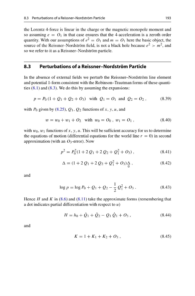
In the absence of external fields we perturb the Reissner–Nordström line element
and potential 1-form consistent with the Robinson–Trautman forms of these quantities (8.1) and (8.3). We do this by assuming the expansions:
p = P 0 (1 + Q 1 + Q 2 + O 3 ) with Q 1 = O 1 and Q 2 = O 2 ,
(8.39)
with P 0 given by (8.25), Q 1 , Q 2 functions of x, y, u, and
w = w 0 + w 1 + O 2 with w 0 = O 0 , w 1 = O 1 ,
(8.40)
with w 0 , w 1 functions of x, y, u. This will be sufficient accuracy for us to determine
the equations of motion (differential equations for the world line r = 0) in second
approximation (with an O 3 -error). Now
p
2
= P
2
0 (1 + 2 Q 1 + 2 Q 2 + Q
2
1 + O 3 ) ,
(8.41)
= (1 + 2 Q 1 + 2 Q 2 + Q
2
1 + O 3 ))
0
,
(8.42)
and
log p = log P 0 + Q 1 + Q 2 −
1
2
Q
2
1 + O 3 .
(8.43)
Hence H and K in (8.6) and (8.11) take the approximate forms (remembering that
a dot indicates partial differentiation with respect to u)
H = h 0 + ˙
Q 1 + ˙
Q 2 − Q 1 ˙
Q 1 + O 3 ,
(8.44)
and
K = 1 + K 1 + K 2 + O 3 ,
(8.45)
193
the Lorentz 4-force is linear in the charge or the magnetic monopole moment and
so assuming e = O 1 in that case ensures that the 4-acceleration is a zeroth order
quantity. With our assumptions of e 2 = O 1 and m = O 1 here the basic object, the
source of the Reissner–Nordström field, is not a black hole because e 2 > m 2 , and
so we refer to it as a Reissner–Nordström particle.
8.3
Perturbations of a Reissner–Nordström Particle
In the absence of external fields we perturb the Reissner–Nordström line element
and potential 1-form consistent with the Robinson–Trautman forms of these quantities (8.1) and (8.3). We do this by assuming the expansions:
p = P 0 (1 + Q 1 + Q 2 + O 3 ) with Q 1 = O 1 and Q 2 = O 2 ,
(8.39)
with P 0 given by (8.25), Q 1 , Q 2 functions of x, y, u, and
w = w 0 + w 1 + O 2 with w 0 = O 0 , w 1 = O 1 ,
(8.40)
with w 0 , w 1 functions of x, y, u. This will be sufficient accuracy for us to determine
the equations of motion (differential equations for the world line r = 0) in second
approximation (with an O 3 -error). Now
p
2
= P
2
0 (1 + 2 Q 1 + 2 Q 2 + Q
2
1 + O 3 ) ,
(8.41)
= (1 + 2 Q 1 + 2 Q 2 + Q
2
1 + O 3 ))
0
,
(8.42)
and
log p = log P 0 + Q 1 + Q 2 −
1
2
Q
2
1 + O 3 .
(8.43)
Hence H and K in (8.6) and (8.11) take the approximate forms (remembering that
a dot indicates partial differentiation with respect to u)
H = h 0 + ˙
Q 1 + ˙
Q 2 − Q 1 ˙
Q 1 + O 3 ,
(8.44)
and
K = 1 + K 1 + K 2 + O 3 ,
(8.45)