

150
6 de Sitter Cosmology
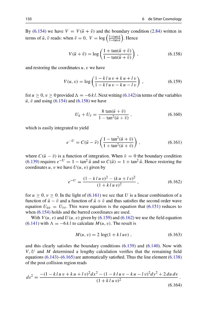
By (6.154) we have V = V ( ¯
u + ¯
v) and the boundary condition (2.84) written in
terms of ¯
u, ¯
v reads: when ¯
v = 0, V = log
1+tan ¯
u
1−tan ¯
u
. Hence
V ( ¯
u + ¯
v) = log
1 + tan( ¯
u + ¯
v)
1 − tan( ¯
u + ¯
v)
,
(6.158)
and restoring the coordinates u, v we have
V (u, v) = log
1 − k l u v + k u + l v
1 − k l u v − k u − l v
,
(6.159)
for u ≥ 0, v ≥ 0 provided = −6 k l. Next writing (6.142) in terms of the variables
¯
u, ¯
v and using (6.154) and (6.158) we have
U ¯
u + U ¯
v =
8 tan( ¯
u + ¯
v)
1 − tan 2 ( ¯
u + ¯
v)
,
(6.160)
which is easily integrated to yield
e
−U
= C( ¯
u − ¯
v)
1 − tan 2 ( ¯
u + ¯
v)
1 + tan 2 ( ¯
u + ¯
v)
,
(6.161)
where C( ¯
u − ¯
v) is a function of integration. When ¯
v = 0 the boundary condition
(6.139) requires e −U = 1 − tan 2 ¯
u and so C( ¯
u) = 1 + tan 2 ¯
u. Hence restoring the
coordinates u, v we have U(u, v) given by
e
−U
=
(1 − k l u v) 2 − (k u + l v) 2
(1 + k l u v) 2
,
(6.162)
for u ≥ 0, v ≥ 0. In the light of (6.161) we see that U is a linear combination of a
function of ¯
u − ¯
v and a function of ¯
u + ¯
v and thus satisfies the second order wave
equation U ¯
u ¯
u = U ¯
v ¯
v . This wave equation is the equation that (6.151) reduces to
when (6.154) holds and the barred coordinates are used.
With V (u, v) and U(u, v) given by (6.159) and (6.162) we use the field equation
(6.141) with = −6 k l to calculate M(u, v). The result is
M(u, v) = 2 log(1 + k l uv) ,
(6.163)
and this clearly satisfies the boundary conditions (6.139) and (6.140). Now with
V , U and M determined a lengthy calculation verifies that the remaining field
equations (6.143)–(6.165) are automatically satisfied. Thus the line element (6.138)
of the post collision region reads
ds
2
=
−(1 − k l u v + k u + l v) 2 dx 2 − (1 − k l u v − k u − l v) 2 dy 2 + 2 du dv
(1 + k l u v) 2
.
(6.164)
6 de Sitter Cosmology
By (6.154) we have V = V ( ¯
u + ¯
v) and the boundary condition (2.84) written in
terms of ¯
u, ¯
v reads: when ¯
v = 0, V = log
1+tan ¯
u
1−tan ¯
u
. Hence
V ( ¯
u + ¯
v) = log
1 + tan( ¯
u + ¯
v)
1 − tan( ¯
u + ¯
v)
,
(6.158)
and restoring the coordinates u, v we have
V (u, v) = log
1 − k l u v + k u + l v
1 − k l u v − k u − l v
,
(6.159)
for u ≥ 0, v ≥ 0 provided = −6 k l. Next writing (6.142) in terms of the variables
¯
u, ¯
v and using (6.154) and (6.158) we have
U ¯
u + U ¯
v =
8 tan( ¯
u + ¯
v)
1 − tan 2 ( ¯
u + ¯
v)
,
(6.160)
which is easily integrated to yield
e
−U
= C( ¯
u − ¯
v)
1 − tan 2 ( ¯
u + ¯
v)
1 + tan 2 ( ¯
u + ¯
v)
,
(6.161)
where C( ¯
u − ¯
v) is a function of integration. When ¯
v = 0 the boundary condition
(6.139) requires e −U = 1 − tan 2 ¯
u and so C( ¯
u) = 1 + tan 2 ¯
u. Hence restoring the
coordinates u, v we have U(u, v) given by
e
−U
=
(1 − k l u v) 2 − (k u + l v) 2
(1 + k l u v) 2
,
(6.162)
for u ≥ 0, v ≥ 0. In the light of (6.161) we see that U is a linear combination of a
function of ¯
u − ¯
v and a function of ¯
u + ¯
v and thus satisfies the second order wave
equation U ¯
u ¯
u = U ¯
v ¯
v . This wave equation is the equation that (6.151) reduces to
when (6.154) holds and the barred coordinates are used.
With V (u, v) and U(u, v) given by (6.159) and (6.162) we use the field equation
(6.141) with = −6 k l to calculate M(u, v). The result is
M(u, v) = 2 log(1 + k l uv) ,
(6.163)
and this clearly satisfies the boundary conditions (6.139) and (6.140). Now with
V , U and M determined a lengthy calculation verifies that the remaining field
equations (6.143)–(6.165) are automatically satisfied. Thus the line element (6.138)
of the post collision region reads
ds
2
=
−(1 − k l u v + k u + l v) 2 dx 2 − (1 − k l u v − k u − l v) 2 dy 2 + 2 du dv
(1 + k l u v) 2
.
(6.164)