

148
6 de Sitter Cosmology
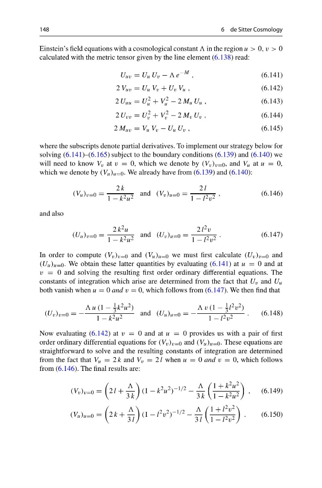
Einstein’s field equations with a cosmological constant in the region u > 0, v > 0
calculated with the metric tensor given by the line element (6.138) read:
U uv = U u U v − e
−M ,
(6.141)
2 V uv = U u V v + U v V u ,
(6.142)
2 U uu = U
2
u + V
2
u − 2 M u U u ,
(6.143)
2 U vv = U
2
v + V
2
v − 2 M v U v ,
(6.144)
2 M uv = V u V v − U u U v ,
(6.145)
where the subscripts denote partial derivatives. To implement our strategy below for
solving (6.141)–(6.165) subject to the boundary conditions (6.139) and (6.140) we
will need to know V v at v = 0, which we denote by (V v ) v=0 , and V u at u = 0,
which we denote by (V u ) u=0 . We already have from (6.139) and (6.140):
(V u ) v=0 =
2 k
1 − k 2 u 2 and (V v ) u=0 =
2 l
1 − l 2 v 2 ,
(6.146)
and also
(U u ) v=0 =
2 k 2 u
1 − k 2 u 2 and (U v ) u=0 =
2 l 2 v
1 − l 2 v 2 .
(6.147)
In order to compute (V v ) v=0 and (V u ) u=0 we must first calculate (U v ) v=0 and
(U u ) u=0 . We obtain these latter quantities by evaluating (6.141) at u = 0 and at
v = 0 and solving the resulting first order ordinary differential equations. The
constants of integration which arise are determined from the fact that U v and U u
both vanish when u = 0 and v = 0, which follows from (6.147). We then find that
(U v ) v=0 = −
u (1 −
1
3 k 2 u 2 )
1 − k 2 u 2
and (U u ) u=0 = −
v (1 −
1
3 l 2 v 2 )
1 − l 2 v 2
.
(6.148)
Now evaluating (6.142) at v = 0 and at u = 0 provides us with a pair of first
order ordinary differential equations for (V v ) v=0 and (V u ) u=0 . These equations are
straightforward to solve and the resulting constants of integration are determined
from the fact that V u = 2 k and V v = 2 l when u = 0 and v = 0, which follows
from (6.146). The final results are:
(V v ) v=0 =
2 l +
3 k
(1 − k
2 u
2 )
−1/2
−
3 k
1 + k 2 u 2
1 − k 2 u 2
, (6.149)
(V u ) u=0 =
2 k +
3 l
(1 − l
2 v
2 )
−1/2
−
3 l
1 + l 2 v 2
1 − l 2 v 2
.
(6.150)
6 de Sitter Cosmology
Einstein’s field equations with a cosmological constant in the region u > 0, v > 0
calculated with the metric tensor given by the line element (6.138) read:
U uv = U u U v − e
−M ,
(6.141)
2 V uv = U u V v + U v V u ,
(6.142)
2 U uu = U
2
u + V
2
u − 2 M u U u ,
(6.143)
2 U vv = U
2
v + V
2
v − 2 M v U v ,
(6.144)
2 M uv = V u V v − U u U v ,
(6.145)
where the subscripts denote partial derivatives. To implement our strategy below for
solving (6.141)–(6.165) subject to the boundary conditions (6.139) and (6.140) we
will need to know V v at v = 0, which we denote by (V v ) v=0 , and V u at u = 0,
which we denote by (V u ) u=0 . We already have from (6.139) and (6.140):
(V u ) v=0 =
2 k
1 − k 2 u 2 and (V v ) u=0 =
2 l
1 − l 2 v 2 ,
(6.146)
and also
(U u ) v=0 =
2 k 2 u
1 − k 2 u 2 and (U v ) u=0 =
2 l 2 v
1 − l 2 v 2 .
(6.147)
In order to compute (V v ) v=0 and (V u ) u=0 we must first calculate (U v ) v=0 and
(U u ) u=0 . We obtain these latter quantities by evaluating (6.141) at u = 0 and at
v = 0 and solving the resulting first order ordinary differential equations. The
constants of integration which arise are determined from the fact that U v and U u
both vanish when u = 0 and v = 0, which follows from (6.147). We then find that
(U v ) v=0 = −
u (1 −
1
3 k 2 u 2 )
1 − k 2 u 2
and (U u ) u=0 = −
v (1 −
1
3 l 2 v 2 )
1 − l 2 v 2
.
(6.148)
Now evaluating (6.142) at v = 0 and at u = 0 provides us with a pair of first
order ordinary differential equations for (V v ) v=0 and (V u ) u=0 . These equations are
straightforward to solve and the resulting constants of integration are determined
from the fact that V u = 2 k and V v = 2 l when u = 0 and v = 0, which follows
from (6.146). The final results are:
(V v ) v=0 =
2 l +
3 k
(1 − k
2 u
2 )
−1/2
−
3 k
1 + k 2 u 2
1 − k 2 u 2
, (6.149)
(V u ) u=0 =
2 k +
3 l
(1 − l
2 v
2 )
−1/2
−
3 l
1 + l 2 v 2
1 − l 2 v 2
.
(6.150)