

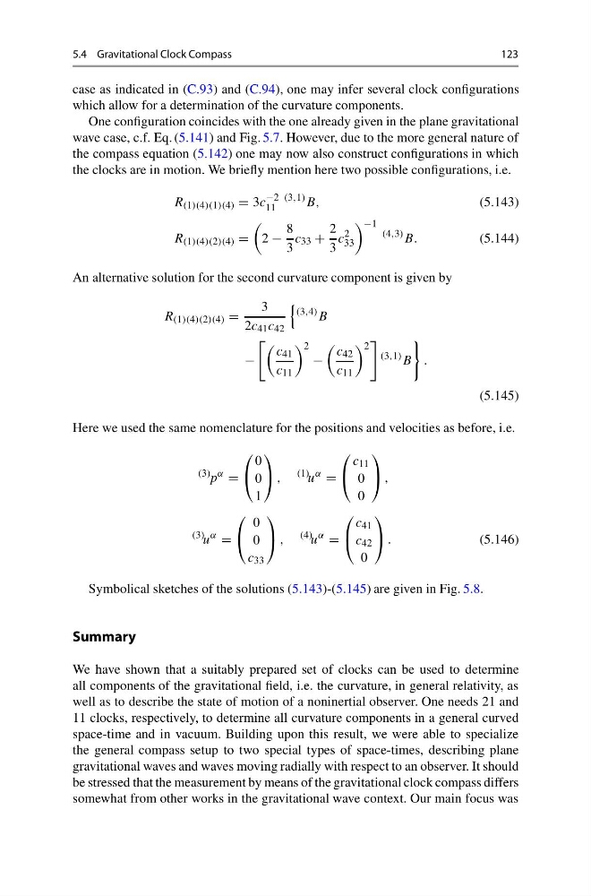
5.4 Gravitational Clock Compass
123
case as indicated in (C.93) and (C.94), one may infer several clock configurations
which allow for a determination of the curvature components.
One configuration coincides with the one already given in the plane gravitational
wave case, c.f. Eq. (5.141) and Fig. 5.7. However, due to the more general nature of
the compass equation (5.142) one may now also construct configurations in which
the clocks are in motion. We briefly mention here two possible configurations, i.e.
R (1)(4)(1)(4) = 3c
−2
11
(3,1) B,
(5.143)
R (1)(4)(2)(4) =
2 −
8
3
c 33 +
2
3
c
2
33
−1
(4,3) B.
(5.144)
An alternative solution for the second curvature component is given by
R (1)(4)(2)(4) =
3
2c 41 c 42
(3,4) B
−
c 41
c 11
2
−
c 42
c 11
2
(3,1) B
.
(5.145)
Here we used the same nomenclature for the positions and velocities as before, i.e.
(3)
p
α
=
⎛
⎝
0
0
1
⎞
⎠ ,
(1)
u
α
=
⎛
⎝
c 11
0
0
⎞
⎠ ,
(3)
u
α
=
⎛
⎝
0
0
c 33
⎞
⎠ ,
(4)
u
α
=
⎛
⎝
c 41
c 42
0
⎞
⎠ .
(5.146)
Symbolical sketches of the solutions (5.143)-(5.145) are given in Fig. 5.8.
Summary
We have shown that a suitably prepared set of clocks can be used to determine
all components of the gravitational field, i.e. the curvature, in general relativity, as
well as to describe the state of motion of a noninertial observer. One needs 21 and
11 clocks, respectively, to determine all curvature components in a general curved
space-time and in vacuum. Building upon this result, we were able to specialize
the general compass setup to two special types of space-times, describing plane
gravitational waves and waves moving radially with respect to an observer. It should
be stressed that the measurement by means of the gravitational clock compass differs
somewhat from other works in the gravitational wave context. Our main focus was
123
case as indicated in (C.93) and (C.94), one may infer several clock configurations
which allow for a determination of the curvature components.
One configuration coincides with the one already given in the plane gravitational
wave case, c.f. Eq. (5.141) and Fig. 5.7. However, due to the more general nature of
the compass equation (5.142) one may now also construct configurations in which
the clocks are in motion. We briefly mention here two possible configurations, i.e.
R (1)(4)(1)(4) = 3c
−2
11
(3,1) B,
(5.143)
R (1)(4)(2)(4) =
2 −
8
3
c 33 +
2
3
c
2
33
−1
(4,3) B.
(5.144)
An alternative solution for the second curvature component is given by
R (1)(4)(2)(4) =
3
2c 41 c 42
(3,4) B
−
c 41
c 11
2
−
c 42
c 11
2
(3,1) B
.
(5.145)
Here we used the same nomenclature for the positions and velocities as before, i.e.
(3)
p
α
=
⎛
⎝
0
0
1
⎞
⎠ ,
(1)
u
α
=
⎛
⎝
c 11
0
0
⎞
⎠ ,
(3)
u
α
=
⎛
⎝
0
0
c 33
⎞
⎠ ,
(4)
u
α
=
⎛
⎝
c 41
c 42
0
⎞
⎠ .
(5.146)
Symbolical sketches of the solutions (5.143)-(5.145) are given in Fig. 5.8.
Summary
We have shown that a suitably prepared set of clocks can be used to determine
all components of the gravitational field, i.e. the curvature, in general relativity, as
well as to describe the state of motion of a noninertial observer. One needs 21 and
11 clocks, respectively, to determine all curvature components in a general curved
space-time and in vacuum. Building upon this result, we were able to specialize
the general compass setup to two special types of space-times, describing plane
gravitational waves and waves moving radially with respect to an observer. It should
be stressed that the measurement by means of the gravitational clock compass differs
somewhat from other works in the gravitational wave context. Our main focus was