

6.6 Nonlinear Modeling Method Based on DBN
233
algorithm are utilized to modify the weights of the network [36, 37]. The structure
of the final network is determined as [38, 39].
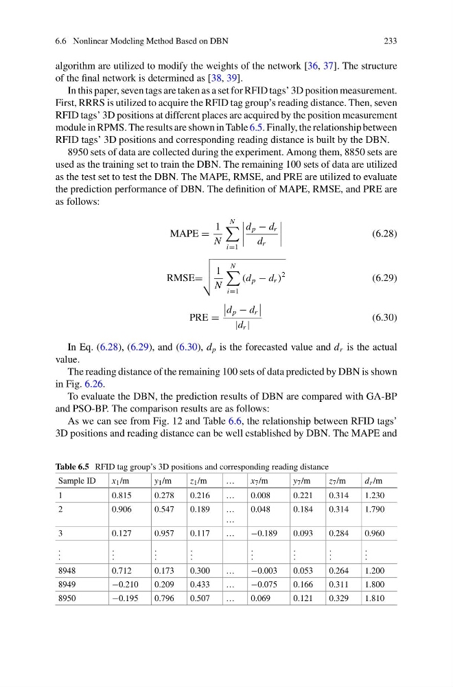
In this paper, seven tags are taken as a set for RFID tags’ 3D position measurement.
First, RRRS is utilized to acquire the RFID tag group’s reading distance. Then, seven
RFID tags’ 3D positions at different places are acquired by the position measurement
module in RPMS. The results are shown in Table 6.5. Finally, the relationship between
RFID tags’ 3D positions and corresponding reading distance is built by the DBN.
8950 sets of data are collected during the experiment. Among them, 8850 sets are
used as the training set to train the DBN. The remaining 100 sets of data are utilized
as the test set to test the DBN. The MAPE, RMSE, and PRE are utilized to evaluate
the prediction performance of DBN. The definition of MAPE, RMSE, and PRE are
as follows:
MAPE =
1
N
N
i=1
d p − d r
d r
(6.28)
RMSE=
1
N
N
i=1
(d p − d r )
2
(6.29)
PRE =
d p − d r
|d r |
(6.30)
In Eq. (6.28), (6.29), and (6.30), d p is the forecasted value and d r is the actual
value.
The reading distance of the remaining 100 sets of data predicted by DBN is shown
in Fig. 6.26.
To evaluate the DBN, the prediction results of DBN are compared with GA-BP
and PSO-BP. The comparison results are as follows:
As we can see from Fig. 12 and Table 6.6, the relationship between RFID tags’
3D positions and reading distance can be well established by DBN. The MAPE and
Table 6.5 RFID tag group’s 3D positions and corresponding reading distance
Sample ID
x 1 /m
y 1 /m
z 1 /m
…
x 7 /m
y 7 /m
z 7 /m
d r /m
1
0.815
0.278
0.216
…
0.008
0.221
0.314
1.230
2
0.906
0.547
0.189
…
…
0.048
0.184
0.314
1.790
3
0.127
0.957
0.117
…
−0.189
0.093
0.284
0.960
. . .
. . .
. . .
. . .
. . .
. . .
. . .
. . .
8948
0.712
0.173
0.300
…
−0.003
0.053
0.264
1.200
8949
−0.210
0.209
0.433
…
−0.075
0.166
0.311
1.800
8950
−0.195
0.796
0.507
…
0.069
0.121
0.329
1.810
233
algorithm are utilized to modify the weights of the network [36, 37]. The structure
of the final network is determined as [38, 39].
In this paper, seven tags are taken as a set for RFID tags’ 3D position measurement.
First, RRRS is utilized to acquire the RFID tag group’s reading distance. Then, seven
RFID tags’ 3D positions at different places are acquired by the position measurement
module in RPMS. The results are shown in Table 6.5. Finally, the relationship between
RFID tags’ 3D positions and corresponding reading distance is built by the DBN.
8950 sets of data are collected during the experiment. Among them, 8850 sets are
used as the training set to train the DBN. The remaining 100 sets of data are utilized
as the test set to test the DBN. The MAPE, RMSE, and PRE are utilized to evaluate
the prediction performance of DBN. The definition of MAPE, RMSE, and PRE are
as follows:
MAPE =
1
N
N
i=1
d p − d r
d r
(6.28)
RMSE=
1
N
N
i=1
(d p − d r )
2
(6.29)
PRE =
d p − d r
|d r |
(6.30)
In Eq. (6.28), (6.29), and (6.30), d p is the forecasted value and d r is the actual
value.
The reading distance of the remaining 100 sets of data predicted by DBN is shown
in Fig. 6.26.
To evaluate the DBN, the prediction results of DBN are compared with GA-BP
and PSO-BP. The comparison results are as follows:
As we can see from Fig. 12 and Table 6.6, the relationship between RFID tags’
3D positions and reading distance can be well established by DBN. The MAPE and
Table 6.5 RFID tag group’s 3D positions and corresponding reading distance
Sample ID
x 1 /m
y 1 /m
z 1 /m
…
x 7 /m
y 7 /m
z 7 /m
d r /m
1
0.815
0.278
0.216
…
0.008
0.221
0.314
1.230
2
0.906
0.547
0.189
…
…
0.048
0.184
0.314
1.790
3
0.127
0.957
0.117
…
−0.189
0.093
0.284
0.960
. . .
. . .
. . .
. . .
. . .
. . .
. . .
. . .
8948
0.712
0.173
0.300
…
−0.003
0.053
0.264
1.200
8949
−0.210
0.209
0.433
…
−0.075
0.166
0.311
1.800
8950
−0.195
0.796
0.507
…
0.069
0.121
0.329
1.810