

Fundamental concepts 15
It can be shown that the transfer matrix given in Eq. (2.14) also satisfies
.
.
(2.16)
For a closed kinematic chain consisting of n links, by repeatedly applying
Eq. (2.13), we have p′ 2 = T 12 p′ 1 , p′ 3 = T 23 p′ 2 , . . ., p′ n = T (n–1)n p′ n–1 and
p′ 1 = T n1 p′ n noting that n + 1 becomes 1 for a closed chain. Combining these
expressions together gives
,
(2.17)
where I is a 4 × 4 unit matrix. Eq. (2.17) can be used to derive the closure
equations of the closed kinematic chain.
The matrix method, like any of the other kinematic methods, takes both
the topology and the geometry of a linkage into account. It can be used to
determine the mobility of a linkage. If Eq. (2.17) has only one or a limited
number of solutions, the closed chain is in fact locked. When one of the
kinematic variables can change freely while the others are found to be
dependent upon it algebraically by the equations in Eq. (2.17), the linkage
has mobility one. If two free kinematic variables exist, the linkage will
have mobility two. The number of mobility of linkages is equal to the
number of free kinematic variables in the closure equations. Meanwhile,
other kinematic properties of the linkages, e.g. motion trajectories, can also
be obtained from the closure equations.
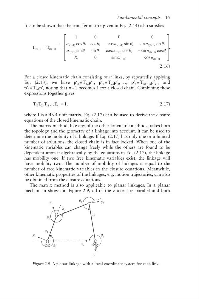
The matrix method is also applicable to planar linkages. In a planar
mechanism shown in Figure 2.9, all of the z axes are parallel and both
Figure 2.9 A planar linkage with a local coordinate system for each link.
It can be shown that the transfer matrix given in Eq. (2.14) also satisfies
.
.
(2.16)
For a closed kinematic chain consisting of n links, by repeatedly applying
Eq. (2.13), we have p′ 2 = T 12 p′ 1 , p′ 3 = T 23 p′ 2 , . . ., p′ n = T (n–1)n p′ n–1 and
p′ 1 = T n1 p′ n noting that n + 1 becomes 1 for a closed chain. Combining these
expressions together gives
,
(2.17)
where I is a 4 × 4 unit matrix. Eq. (2.17) can be used to derive the closure
equations of the closed kinematic chain.
The matrix method, like any of the other kinematic methods, takes both
the topology and the geometry of a linkage into account. It can be used to
determine the mobility of a linkage. If Eq. (2.17) has only one or a limited
number of solutions, the closed chain is in fact locked. When one of the
kinematic variables can change freely while the others are found to be
dependent upon it algebraically by the equations in Eq. (2.17), the linkage
has mobility one. If two free kinematic variables exist, the linkage will
have mobility two. The number of mobility of linkages is equal to the
number of free kinematic variables in the closure equations. Meanwhile,
other kinematic properties of the linkages, e.g. motion trajectories, can also
be obtained from the closure equations.
The matrix method is also applicable to planar linkages. In a planar
mechanism shown in Figure 2.9, all of the z axes are parallel and both
Figure 2.9 A planar linkage with a local coordinate system for each link.