

8
1 Introduction
1.3.2 Two-Fluid Model
Two-fluid models apply a Eulerian framework that threats mathematically both the
gas and solid phase as fully interpenetrating continua via interphase momentum
exchanges, allowing one to simulate macroscopic dynamics at a relatively low cost.
The hydrodynamic equations comprise of continuity and momentum equations, given
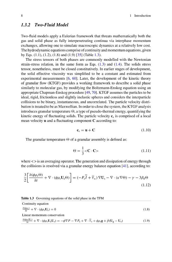
by Eqs. (1.1), (1.2), (1.8) and (1.9) [35] (Table 1.3).
The stress tensors of both phases are commonly modelled with the Newtonian
strain-stress relation, in the same form as Eqs. (1.3) and (1.4). The solids stress
tensor, nonetheless, must be closed constitutively. In earlier stages of development,
the solid effective viscosity was simplified to be a constant and estimated from
experimental measurements [6, 60]. Later, the development of the kinetic theory
of granular flow (KTGF) provides a working framework to describe a solid phase
similarly to molecular gas, by modifying the Boltzmann-Enskog equation using an
appropriate Chapman-Enskog procedure [49, 70]. KTGF assumes the particles to be
ideal, rigid, frictionless and slightly inelastic spheres and considers the interparticle
collisions to be binary, instantaneous, and uncorrelated. The particle velocity distribution is treated to be as Maxwellian. In order to close the system, the KTGF analysis
introduces granular temperature , a type of pseudo-thermal energy, quantifying the
kinetic energy of fluctuating solids. The particle velocity c s is comprised of a local
mean velocity u and a fluctuating component C according to:
c s = u + C
(1.10)
The granular temperature of a granular assembly is defined as:
=
1
3
(1.11)
where < > is an averaging operator. The generation and dissipation of energy through
the collisions is resolved via a granular energy balance equation [41], according to:
3
2
∂(φρ s )
∂t
+ ∇ · (φρ s U s )
= (−P s I + τ s: ) ∇U s − ∇ · (κ∇) − γ − 3β d
(1.12)
Table 1.3 Governing equations of the solid phase in the TFM
Continuity equation
∂(φρs)
∂t + ∇ · (φρ s U s ) = 0
(1.8)
Linear momentum conservation
∂(φρsUs)
∂t
+ ∇ · (φρ s U s U s ) = −φ∇ P − ∇ P s + ∇ · τ s + φρ s g + β(U g − U s )
(1.9)
1 Introduction
1.3.2 Two-Fluid Model
Two-fluid models apply a Eulerian framework that threats mathematically both the
gas and solid phase as fully interpenetrating continua via interphase momentum
exchanges, allowing one to simulate macroscopic dynamics at a relatively low cost.
The hydrodynamic equations comprise of continuity and momentum equations, given
by Eqs. (1.1), (1.2), (1.8) and (1.9) [35] (Table 1.3).
The stress tensors of both phases are commonly modelled with the Newtonian
strain-stress relation, in the same form as Eqs. (1.3) and (1.4). The solids stress
tensor, nonetheless, must be closed constitutively. In earlier stages of development,
the solid effective viscosity was simplified to be a constant and estimated from
experimental measurements [6, 60]. Later, the development of the kinetic theory
of granular flow (KTGF) provides a working framework to describe a solid phase
similarly to molecular gas, by modifying the Boltzmann-Enskog equation using an
appropriate Chapman-Enskog procedure [49, 70]. KTGF assumes the particles to be
ideal, rigid, frictionless and slightly inelastic spheres and considers the interparticle
collisions to be binary, instantaneous, and uncorrelated. The particle velocity distribution is treated to be as Maxwellian. In order to close the system, the KTGF analysis
introduces granular temperature , a type of pseudo-thermal energy, quantifying the
kinetic energy of fluctuating solids. The particle velocity c s is comprised of a local
mean velocity u and a fluctuating component C according to:
c s = u + C
(1.10)
The granular temperature of a granular assembly is defined as:
=
1
3
(1.11)
where < > is an averaging operator. The generation and dissipation of energy through
the collisions is resolved via a granular energy balance equation [41], according to:
3
2
∂(φρ s )
∂t
+ ∇ · (φρ s U s )
= (−P s I + τ s: ) ∇U s − ∇ · (κ∇) − γ − 3β d
(1.12)
Table 1.3 Governing equations of the solid phase in the TFM
Continuity equation
∂(φρs)
∂t + ∇ · (φρ s U s ) = 0
(1.8)
Linear momentum conservation
∂(φρsUs)
∂t
+ ∇ · (φρ s U s U s ) = −φ∇ P − ∇ P s + ∇ · τ s + φρ s g + β(U g − U s )
(1.9)