

134
5 The Role of Solid Mechanics in Stabilising Structured Flows
Fig. 5.17 Solid circulation patterns at ϕ = 0 for a D5-1 (μ f = 0.1), b D5-2 (μ f = 0.2) and c D5-3
(μ f = 0.3)
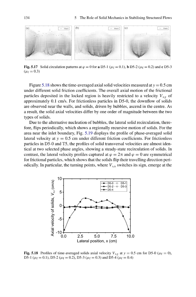
Figure 5.18 shows the time-averaged axial solid velocities measured at y = 0.5 cm
under different solid friction coefficients. The overall axial motion of the frictional
particles deposited in the locked region is heavily restricted to a velocity V s,y of
approximately 0.1 cm/s. For frictionless particles in D5-0, the downflow of solids
are observed near the walls, and solids, driven by bubbles, ascend in the centre. As
a result, the solid axial velocities differ by one order of magnitude between the two
types of solids.
Due to the alternative nucleation of bubbles, the lateral solid recirculation, therefore, flips periodically, which shows a regionally recursive motion of solids. For the
area near the inlet boundary, Fig. 5.19 displays the profile of phase-averaged solid
lateral velocity at y = 0.5 cm under different friction coefficients. For frictionless
particles in D5-0 and T5, the profiles of solid transversal velocities are almost identical at two selected phase angles, showing a steady-state recirculation of solids. In
contrast, the lateral velocity profiles captured at ϕ = 2π and ϕ = 0 are symmetrical
for frictional particles, which shows that the solids flip their travelling direction periodically. In particular, the turning points, where V s,x switches its sign, emerge at the
0.0
2.5
5.0
7.5
10.0
-10
-5
0
5
10
Axial velocity of solids, V
s,y (cm/s)
Lateral position, x (cm)
D5-0
D5-1
D5-2
D5-3
D5-4
Fig. 5.18 Profiles of time-averaged solids axial velocity V s,y at y = 0.5 cm for D5-0 (μ f = 0),
D5-1 (μ f = 0.1), D5-2 (μ f = 0.2), D5-3 (μ f = 0.3) and D5-4 (μ f = 0.4)
5 The Role of Solid Mechanics in Stabilising Structured Flows
Fig. 5.17 Solid circulation patterns at ϕ = 0 for a D5-1 (μ f = 0.1), b D5-2 (μ f = 0.2) and c D5-3
(μ f = 0.3)
Figure 5.18 shows the time-averaged axial solid velocities measured at y = 0.5 cm
under different solid friction coefficients. The overall axial motion of the frictional
particles deposited in the locked region is heavily restricted to a velocity V s,y of
approximately 0.1 cm/s. For frictionless particles in D5-0, the downflow of solids
are observed near the walls, and solids, driven by bubbles, ascend in the centre. As
a result, the solid axial velocities differ by one order of magnitude between the two
types of solids.
Due to the alternative nucleation of bubbles, the lateral solid recirculation, therefore, flips periodically, which shows a regionally recursive motion of solids. For the
area near the inlet boundary, Fig. 5.19 displays the profile of phase-averaged solid
lateral velocity at y = 0.5 cm under different friction coefficients. For frictionless
particles in D5-0 and T5, the profiles of solid transversal velocities are almost identical at two selected phase angles, showing a steady-state recirculation of solids. In
contrast, the lateral velocity profiles captured at ϕ = 2π and ϕ = 0 are symmetrical
for frictional particles, which shows that the solids flip their travelling direction periodically. In particular, the turning points, where V s,x switches its sign, emerge at the
0.0
2.5
5.0
7.5
10.0
-10
-5
0
5
10
Axial velocity of solids, V
s,y (cm/s)
Lateral position, x (cm)
D5-0
D5-1
D5-2
D5-3
D5-4
Fig. 5.18 Profiles of time-averaged solids axial velocity V s,y at y = 0.5 cm for D5-0 (μ f = 0),
D5-1 (μ f = 0.1), D5-2 (μ f = 0.2), D5-3 (μ f = 0.3) and D5-4 (μ f = 0.4)