

5.4 Bubble Recognition and Analysis
119
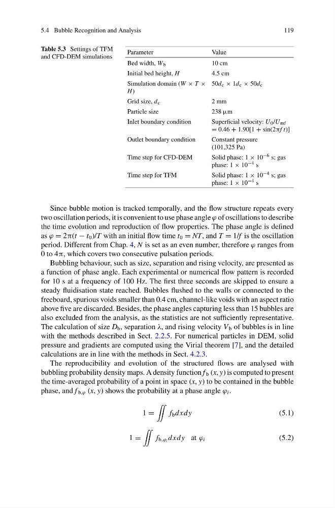
Table 5.3 Settings of TFM
and CFD-DEM simulations
Parameter
Value
Bed width, W b
10 cm
Initial bed height, H
4.5 cm
Simulation domain (W × T ×
H)
50d c × 1d c × 50d c
Grid size, d c
2 mm
Particle size
238 μm
Inlet boundary condition
Superficial velocity: U 0 /U mf
= 0.46 + 1.90[1 + sin(2πf t)]
Outlet boundary condition
Constant pressure
(101,325 Pa)
Time step for CFD-DEM
Solid phase: 1 × 10 −6 s; gas
phase: 1 × 10 −4 s
Time step for TFM
Solid phase: 1 × 10 −4 s; gas
phase: 1 × 10 −4 s
Since bubble motion is tracked temporally, and the flow structure repeats every
two oscillation periods, it is convenient to use phase angle ϕ of oscillations to describe
the time evolution and reproduction of flow properties. The phase angle is defined
as ϕ = 2π(t − t 0 )/T with an initial flow time t 0 = NT, and T = 1/f is the oscillation
period. Different from Chap. 4, N is set as an even number, therefore ϕ ranges from
0 to 4π, which covers two consecutive pulsation periods.
Bubbling behaviour, such as size, separation and rising velocity, are presented as
a function of phase angle. Each experimental or numerical flow pattern is recorded
for 10 s at a frequency of 100 Hz. The first three seconds are skipped to ensure a
steady fluidisation state reached. Bubbles flushed to the walls or connected to the
freeboard, spurious voids smaller than 0.4 cm, channel-like voids with an aspect ratio
above five are discarded. Besides, the phase angles capturing less than 15 bubbles are
also excluded from the analysis, as the statistics are not sufficiently representative.
The calculation of size D b , separation λ, and rising velocity V b of bubbles is in line
with the methods described in Sect. 2.2.5. For numerical particles in DEM, solid
pressure and gradients are computed using the Virial theorem [7], and the detailed
calculations are in line with the methods in Sect. 4.2.3.
The reproducibility and evolution of the structured flows are analysed with
bubbling probability density maps. A density function f b (x, y) is computed to present
the time-averaged probability of a point in space (x, y) to be contained in the bubble
phase, and f b,ϕ (x, y) shows the probability at a phase angle ϕ i .
1 =
¨
f b dxdy
(5.1)
1 =
¨
f b,ϕ i dxdy at ϕ i
(5.2)
119
Table 5.3 Settings of TFM
and CFD-DEM simulations
Parameter
Value
Bed width, W b
10 cm
Initial bed height, H
4.5 cm
Simulation domain (W × T ×
H)
50d c × 1d c × 50d c
Grid size, d c
2 mm
Particle size
238 μm
Inlet boundary condition
Superficial velocity: U 0 /U mf
= 0.46 + 1.90[1 + sin(2πf t)]
Outlet boundary condition
Constant pressure
(101,325 Pa)
Time step for CFD-DEM
Solid phase: 1 × 10 −6 s; gas
phase: 1 × 10 −4 s
Time step for TFM
Solid phase: 1 × 10 −4 s; gas
phase: 1 × 10 −4 s
Since bubble motion is tracked temporally, and the flow structure repeats every
two oscillation periods, it is convenient to use phase angle ϕ of oscillations to describe
the time evolution and reproduction of flow properties. The phase angle is defined
as ϕ = 2π(t − t 0 )/T with an initial flow time t 0 = NT, and T = 1/f is the oscillation
period. Different from Chap. 4, N is set as an even number, therefore ϕ ranges from
0 to 4π, which covers two consecutive pulsation periods.
Bubbling behaviour, such as size, separation and rising velocity, are presented as
a function of phase angle. Each experimental or numerical flow pattern is recorded
for 10 s at a frequency of 100 Hz. The first three seconds are skipped to ensure a
steady fluidisation state reached. Bubbles flushed to the walls or connected to the
freeboard, spurious voids smaller than 0.4 cm, channel-like voids with an aspect ratio
above five are discarded. Besides, the phase angles capturing less than 15 bubbles are
also excluded from the analysis, as the statistics are not sufficiently representative.
The calculation of size D b , separation λ, and rising velocity V b of bubbles is in line
with the methods described in Sect. 2.2.5. For numerical particles in DEM, solid
pressure and gradients are computed using the Virial theorem [7], and the detailed
calculations are in line with the methods in Sect. 4.2.3.
The reproducibility and evolution of the structured flows are analysed with
bubbling probability density maps. A density function f b (x, y) is computed to present
the time-averaged probability of a point in space (x, y) to be contained in the bubble
phase, and f b,ϕ (x, y) shows the probability at a phase angle ϕ i .
1 =
¨
f b dxdy
(5.1)
1 =
¨
f b,ϕ i dxdy at ϕ i
(5.2)