

118
5 The Role of Solid Mechanics in Stabilising Structured Flows
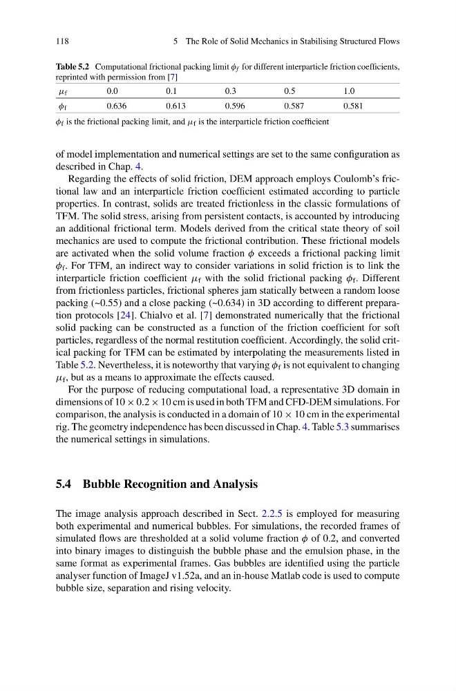
Table 5.2 Computational frictional packing limit φ f for different interparticle friction coefficients,
reprinted with permission from [7]
μ f
0.0
0.1
0.3
0.5
1.0
φ f
0.636
0.613
0.596
0.587
0.581
φ f is the frictional packing limit, and μ f is the interparticle friction coefficient
of model implementation and numerical settings are set to the same configuration as
described in Chap. 4.
Regarding the effects of solid friction, DEM approach employs Coulomb’s frictional law and an interparticle friction coefficient estimated according to particle
properties. In contrast, solids are treated frictionless in the classic formulations of
TFM. The solid stress, arising from persistent contacts, is accounted by introducing
an additional frictional term. Models derived from the critical state theory of soil
mechanics are used to compute the frictional contribution. These frictional models
are activated when the solid volume fraction φ exceeds a frictional packing limit
φ f . For TFM, an indirect way to consider variations in solid friction is to link the
interparticle friction coefficient μ f with the solid frictional packing φ f . Different
from frictionless particles, frictional spheres jam statically between a random loose
packing (~0.55) and a close packing (~0.634) in 3D according to different preparation protocols [24]. Chialvo et al. [7] demonstrated numerically that the frictional
solid packing can be constructed as a function of the friction coefficient for soft
particles, regardless of the normal restitution coefficient. Accordingly, the solid critical packing for TFM can be estimated by interpolating the measurements listed in
Table 5.2. Nevertheless, it is noteworthy that varying φ f is not equivalent to changing
μ f , but as a means to approximate the effects caused.
For the purpose of reducing computational load, a representative 3D domain in
dimensions of 10 × 0.2 × 10 cm is used in both TFM and CFD-DEM simulations. For
comparison, the analysis is conducted in a domain of 10 × 10 cm in the experimental
rig. The geometry independence has been discussed in Chap. 4. Table 5.3 summarises
the numerical settings in simulations.
5.4 Bubble Recognition and Analysis
The image analysis approach described in Sect. 2.2.5 is employed for measuring
both experimental and numerical bubbles. For simulations, the recorded frames of
simulated flows are thresholded at a solid volume fraction φ of 0.2, and converted
into binary images to distinguish the bubble phase and the emulsion phase, in the
same format as experimental frames. Gas bubbles are identified using the particle
analyser function of ImageJ v1.52a, and an in-house Matlab code is used to compute
bubble size, separation and rising velocity.
5 The Role of Solid Mechanics in Stabilising Structured Flows
Table 5.2 Computational frictional packing limit φ f for different interparticle friction coefficients,
reprinted with permission from [7]
μ f
0.0
0.1
0.3
0.5
1.0
φ f
0.636
0.613
0.596
0.587
0.581
φ f is the frictional packing limit, and μ f is the interparticle friction coefficient
of model implementation and numerical settings are set to the same configuration as
described in Chap. 4.
Regarding the effects of solid friction, DEM approach employs Coulomb’s frictional law and an interparticle friction coefficient estimated according to particle
properties. In contrast, solids are treated frictionless in the classic formulations of
TFM. The solid stress, arising from persistent contacts, is accounted by introducing
an additional frictional term. Models derived from the critical state theory of soil
mechanics are used to compute the frictional contribution. These frictional models
are activated when the solid volume fraction φ exceeds a frictional packing limit
φ f . For TFM, an indirect way to consider variations in solid friction is to link the
interparticle friction coefficient μ f with the solid frictional packing φ f . Different
from frictionless particles, frictional spheres jam statically between a random loose
packing (~0.55) and a close packing (~0.634) in 3D according to different preparation protocols [24]. Chialvo et al. [7] demonstrated numerically that the frictional
solid packing can be constructed as a function of the friction coefficient for soft
particles, regardless of the normal restitution coefficient. Accordingly, the solid critical packing for TFM can be estimated by interpolating the measurements listed in
Table 5.2. Nevertheless, it is noteworthy that varying φ f is not equivalent to changing
μ f , but as a means to approximate the effects caused.
For the purpose of reducing computational load, a representative 3D domain in
dimensions of 10 × 0.2 × 10 cm is used in both TFM and CFD-DEM simulations. For
comparison, the analysis is conducted in a domain of 10 × 10 cm in the experimental
rig. The geometry independence has been discussed in Chap. 4. Table 5.3 summarises
the numerical settings in simulations.
5.4 Bubble Recognition and Analysis
The image analysis approach described in Sect. 2.2.5 is employed for measuring
both experimental and numerical bubbles. For simulations, the recorded frames of
simulated flows are thresholded at a solid volume fraction φ of 0.2, and converted
into binary images to distinguish the bubble phase and the emulsion phase, in the
same format as experimental frames. Gas bubbles are identified using the particle
analyser function of ImageJ v1.52a, and an in-house Matlab code is used to compute
bubble size, separation and rising velocity.