

106
4 Modelling Dynamically Structured Fluidisation
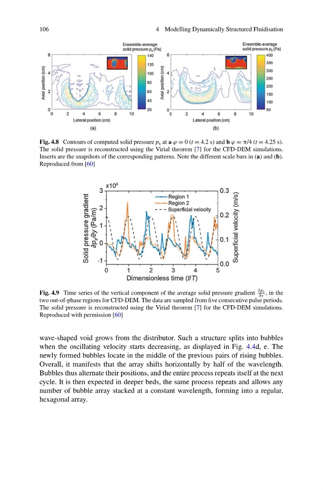
Fig. 4.8 Contours of computed solid pressure p s at a ϕ = 0 (t = 4.2 s) and b ϕ = π/4 (t = 4.25 s).
The solid pressure is reconstructed using the Virial theorem [7] for the CFD-DEM simulations.
Inserts are the snapshots of the corresponding patterns. Note the different scale bars in (a) and (b).
Reproduced from [60]
Fig. 4.9 Time series of the vertical component of the average solid pressure gradient
∂ ps
∂ y , in the
two out-of-phase regions for CFD-DEM. The data are sampled from five consecutive pulse periods.
The solid pressure is reconstructed using the Virial theorem [7] for the CFD-DEM simulations.
Reproduced with permission [60]
wave-shaped void grows from the distributor. Such a structure splits into bubbles
when the oscillating velocity starts decreasing, as displayed in Fig. 4.4d, e. The
newly formed bubbles locate in the middle of the previous pairs of rising bubbles.
Overall, it manifests that the array shifts horizontally by half of the wavelength.
Bubbles thus alternate their positions, and the entire process repeats itself at the next
cycle. It is then expected in deeper beds, the same process repeats and allows any
number of bubble array stacked at a constant wavelength, forming into a regular,
hexagonal array.
4 Modelling Dynamically Structured Fluidisation
Fig. 4.8 Contours of computed solid pressure p s at a ϕ = 0 (t = 4.2 s) and b ϕ = π/4 (t = 4.25 s).
The solid pressure is reconstructed using the Virial theorem [7] for the CFD-DEM simulations.
Inserts are the snapshots of the corresponding patterns. Note the different scale bars in (a) and (b).
Reproduced from [60]
Fig. 4.9 Time series of the vertical component of the average solid pressure gradient
∂ ps
∂ y , in the
two out-of-phase regions for CFD-DEM. The data are sampled from five consecutive pulse periods.
The solid pressure is reconstructed using the Virial theorem [7] for the CFD-DEM simulations.
Reproduced with permission [60]
wave-shaped void grows from the distributor. Such a structure splits into bubbles
when the oscillating velocity starts decreasing, as displayed in Fig. 4.4d, e. The
newly formed bubbles locate in the middle of the previous pairs of rising bubbles.
Overall, it manifests that the array shifts horizontally by half of the wavelength.
Bubbles thus alternate their positions, and the entire process repeats itself at the next
cycle. It is then expected in deeper beds, the same process repeats and allows any
number of bubble array stacked at a constant wavelength, forming into a regular,
hexagonal array.