

100
4 Modelling Dynamically Structured Fluidisation
The variation in the solid volume fraction indicates that a steady state is reached
after 3 s. Bubble identification is therefore carried out between 3 and 10 s at the
post-processing stage of each time step. The wavelength is measured as the distance
between each pair of bubbles nucleated during the same cycle. In the present work,
average properties are used to present for both bubble size and wavelength.
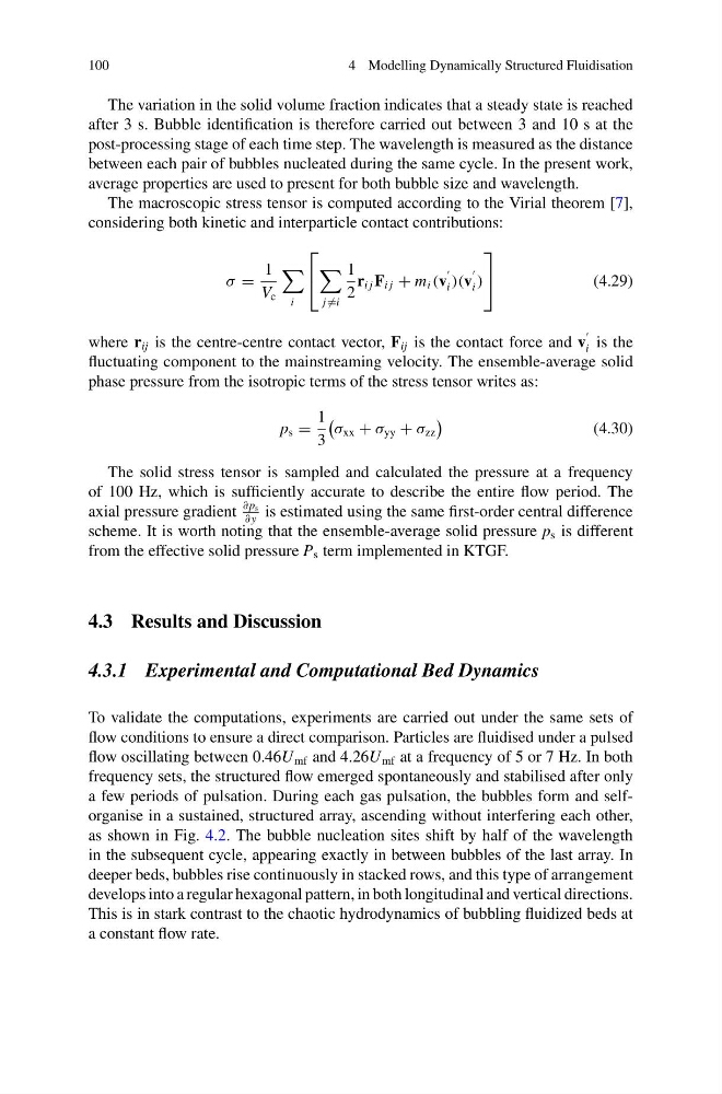
The macroscopic stress tensor is computed according to the Virial theorem [7],
considering both kinetic and interparticle contact contributions:
σ =
1
V c
i
⎡
⎣
j =i
1
2
r i j F i j + m i (v
i )(v
i )
⎤
⎦
(4.29)
where r ij is the centre-centre contact vector, F ij is the contact force and v
i is the
fluctuating component to the mainstreaming velocity. The ensemble-average solid
phase pressure from the isotropic terms of the stress tensor writes as:
p s =
1
3
σ xx + σ yy + σ zz
(4.30)
The solid stress tensor is sampled and calculated the pressure at a frequency
of 100 Hz, which is sufficiently accurate to describe the entire flow period. The
axial pressure gradient
∂ p s
∂ y
is estimated using the same first-order central difference
scheme. It is worth noting that the ensemble-average solid pressure p s is different
from the effective solid pressure P s term implemented in KTGF.
4.3 Results and Discussion
4.3.1 Experimental and Computational Bed Dynamics
To validate the computations, experiments are carried out under the same sets of
flow conditions to ensure a direct comparison. Particles are fluidised under a pulsed
flow oscillating between 0.46U mf and 4.26U mf at a frequency of 5 or 7 Hz. In both
frequency sets, the structured flow emerged spontaneously and stabilised after only
a few periods of pulsation. During each gas pulsation, the bubbles form and selforganise in a sustained, structured array, ascending without interfering each other,
as shown in Fig. 4.2. The bubble nucleation sites shift by half of the wavelength
in the subsequent cycle, appearing exactly in between bubbles of the last array. In
deeper beds, bubbles rise continuously in stacked rows, and this type of arrangement
develops into a regular hexagonal pattern, in both longitudinal and vertical directions.
This is in stark contrast to the chaotic hydrodynamics of bubbling fluidized beds at
a constant flow rate.
4 Modelling Dynamically Structured Fluidisation
The variation in the solid volume fraction indicates that a steady state is reached
after 3 s. Bubble identification is therefore carried out between 3 and 10 s at the
post-processing stage of each time step. The wavelength is measured as the distance
between each pair of bubbles nucleated during the same cycle. In the present work,
average properties are used to present for both bubble size and wavelength.
The macroscopic stress tensor is computed according to the Virial theorem [7],
considering both kinetic and interparticle contact contributions:
σ =
1
V c
i
⎡
⎣
j =i
1
2
r i j F i j + m i (v
i )(v
i )
⎤
⎦
(4.29)
where r ij is the centre-centre contact vector, F ij is the contact force and v
i is the
fluctuating component to the mainstreaming velocity. The ensemble-average solid
phase pressure from the isotropic terms of the stress tensor writes as:
p s =
1
3
σ xx + σ yy + σ zz
(4.30)
The solid stress tensor is sampled and calculated the pressure at a frequency
of 100 Hz, which is sufficiently accurate to describe the entire flow period. The
axial pressure gradient
∂ p s
∂ y
is estimated using the same first-order central difference
scheme. It is worth noting that the ensemble-average solid pressure p s is different
from the effective solid pressure P s term implemented in KTGF.
4.3 Results and Discussion
4.3.1 Experimental and Computational Bed Dynamics
To validate the computations, experiments are carried out under the same sets of
flow conditions to ensure a direct comparison. Particles are fluidised under a pulsed
flow oscillating between 0.46U mf and 4.26U mf at a frequency of 5 or 7 Hz. In both
frequency sets, the structured flow emerged spontaneously and stabilised after only
a few periods of pulsation. During each gas pulsation, the bubbles form and selforganise in a sustained, structured array, ascending without interfering each other,
as shown in Fig. 4.2. The bubble nucleation sites shift by half of the wavelength
in the subsequent cycle, appearing exactly in between bubbles of the last array. In
deeper beds, bubbles rise continuously in stacked rows, and this type of arrangement
develops into a regular hexagonal pattern, in both longitudinal and vertical directions.
This is in stark contrast to the chaotic hydrodynamics of bubbling fluidized beds at
a constant flow rate.