

94
4 Modelling Dynamically Structured Fluidisation
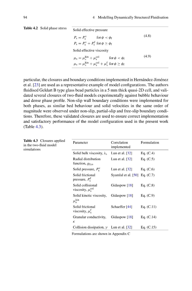
Table 4.2 Solid phase stress
Solid effective pressure
P s = P v
s
for φ < φ f
P s = P v
s + P f
s for φ ≥ φ f
(4.8)
Solid effective viscosity
μ s = μ kin
s + μ col
s
for φ < φ f
μ s = μ kin
s + μ col
s + μ f
s for φ ≥ φ f
(4.9)
particular, the closures and boundary conditions implemented in Hernández-Jiménez
et al. [23] are used as a representative example of model configurations. The authors
fluidised Geldart B type glass bead particles in a 5 mm thick quasi-2D cell, and validated several closures of two-fluid models experimentally against bubble behaviour
and dense phase profile. Non-slip wall boundary conditions were implemented for
both phases, as similar bed behaviour and solid velocities in the same order of
magnitude were observed under non-slip, partial-slip and free-slip boundary conditions. Therefore, these validated closures are used to ensure correct implementation
and satisfactory performance of the model configuration used in the present work
(Table 4.3).
Table 4.3 Closures applied
in the two-fluid model
simulations
Parameter
Correlation
implemented
Formulation
Solid bulk viscosity, λ s Lun et al. [32]
Eq.(C.4)
Radial distribution
function, g 0,ss
Lun et al. [32]
Eq.(C.5)
Solid pressure, P v
s
Lun et al. [32]
Eq.(C.6)
Solid frictional
pressure, P f
s
Syamlal et al. [50] Eq. (C.7)
Solid collisional
viscosity, μ col
s
Gidaspow [18]
Eq.(C.8)
Solid kinetic viscosity,
μ kin
s
Gidaspow [18]
Eq.(C.9)
Solid frictional
viscosity, μ f
s
Schaeffer [44]
Eq. (C.11)
Granular conductivity,
κ
Gidaspow [18]
Eq. (C.14)
Collision dissipation, γ Lun et al. [32]
Eq. (C.15)
Formulations are shown in Appendix C
4 Modelling Dynamically Structured Fluidisation
Table 4.2 Solid phase stress
Solid effective pressure
P s = P v
s
for φ < φ f
P s = P v
s + P f
s for φ ≥ φ f
(4.8)
Solid effective viscosity
μ s = μ kin
s + μ col
s
for φ < φ f
μ s = μ kin
s + μ col
s + μ f
s for φ ≥ φ f
(4.9)
particular, the closures and boundary conditions implemented in Hernández-Jiménez
et al. [23] are used as a representative example of model configurations. The authors
fluidised Geldart B type glass bead particles in a 5 mm thick quasi-2D cell, and validated several closures of two-fluid models experimentally against bubble behaviour
and dense phase profile. Non-slip wall boundary conditions were implemented for
both phases, as similar bed behaviour and solid velocities in the same order of
magnitude were observed under non-slip, partial-slip and free-slip boundary conditions. Therefore, these validated closures are used to ensure correct implementation
and satisfactory performance of the model configuration used in the present work
(Table 4.3).
Table 4.3 Closures applied
in the two-fluid model
simulations
Parameter
Correlation
implemented
Formulation
Solid bulk viscosity, λ s Lun et al. [32]
Eq.(C.4)
Radial distribution
function, g 0,ss
Lun et al. [32]
Eq.(C.5)
Solid pressure, P v
s
Lun et al. [32]
Eq.(C.6)
Solid frictional
pressure, P f
s
Syamlal et al. [50] Eq. (C.7)
Solid collisional
viscosity, μ col
s
Gidaspow [18]
Eq.(C.8)
Solid kinetic viscosity,
μ kin
s
Gidaspow [18]
Eq.(C.9)
Solid frictional
viscosity, μ f
s
Schaeffer [44]
Eq. (C.11)
Granular conductivity,
κ
Gidaspow [18]
Eq. (C.14)
Collision dissipation, γ Lun et al. [32]
Eq. (C.15)
Formulations are shown in Appendix C