

276
P. Torruella et al.
the 4D dataset containing both structural and compositional information of a threedimensional sample). Although the obtained results proved the successful implementation of this technique, allowing even the recovery of ELNES features from the
reconstructed SV, there is clearly room for further improvements.
The separation of spectral components with physical meaningful information
and suitable for tomographic reconstruction remains the main issue in the standard
process described for EELS-SV recovery. Up to now, a combination of PCA (signal
denoising) and ICA or BLU (BSS technique) has been used as the core of the MVA
approximation for data treatment of the EELS-SI datasets. Although these methods
have so far yielded good results, they rely on the ability of the scientist to make
a physical interpretation of the output components, something that is not always
straightforward. Hence, the implementation of clustering (or cluster analysis) to
EELS SV recovery is considered.
11.3.1 Clustering Analysis: Mathematical Principles
An EELS-SI of n = X · Y pixels and E = p channels per spectra can be represented
by a n × p matrix, each spectrum a different row. Any given clustering algorithm will
try to group spectra according to the similarity of their characteristic features (e.g.
position of a certain intensity edge, or intensity ratios for edges in the same positions).
Many options for the clustering implementation, such as K-means [48], densitybased methods, [49] and agglomerative clustering algorithms [50] are available. In
this case, the implementation of the hierarchical agglomerative clustering (HAC) for
the segmentation of EELS-SI is briefly described, following the work done in [45].
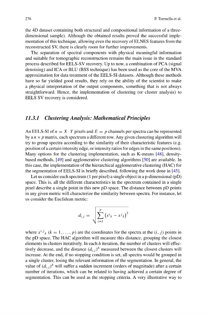
Let us consider each spectrum (1 per pixel) a single object in a p-dimensional (pD)
space. This is, all the different characteristics in the spectrum contained in a single
pixel describe a single point in this new pD space. The distance between pD points
in any given metric will characterize the similarity between spectra. For instance, let
us consider the Euclidean metric:
d i, j =
p
i=1
x i k − x j k
2
where x
i, j
k (k = 1, . . . , p) are the coordinates for the spectra at the (i, j) points in
the pD space. The HAC algorithm will measure this distance, grouping the closest
elements in clusters iteratively. In each h iteration, the number of clusters will effectively decrease, and the distance (d i, j )
h measured between the closest clusters will
increase. At the end, if no stopping condition is set, all spectra would be grouped in
a single cluster, losing the relevant information of the segmentation. In general, the
value of (d i, j )
h will suffer a sudden increment (orders of magnitude) after a certain
number of iterations, which can be related to having achieved a certain degree of
segmentation. This can be used as the stopping criteria. A very illustrative way to
P. Torruella et al.
the 4D dataset containing both structural and compositional information of a threedimensional sample). Although the obtained results proved the successful implementation of this technique, allowing even the recovery of ELNES features from the
reconstructed SV, there is clearly room for further improvements.
The separation of spectral components with physical meaningful information
and suitable for tomographic reconstruction remains the main issue in the standard
process described for EELS-SV recovery. Up to now, a combination of PCA (signal
denoising) and ICA or BLU (BSS technique) has been used as the core of the MVA
approximation for data treatment of the EELS-SI datasets. Although these methods
have so far yielded good results, they rely on the ability of the scientist to make
a physical interpretation of the output components, something that is not always
straightforward. Hence, the implementation of clustering (or cluster analysis) to
EELS SV recovery is considered.
11.3.1 Clustering Analysis: Mathematical Principles
An EELS-SI of n = X · Y pixels and E = p channels per spectra can be represented
by a n × p matrix, each spectrum a different row. Any given clustering algorithm will
try to group spectra according to the similarity of their characteristic features (e.g.
position of a certain intensity edge, or intensity ratios for edges in the same positions).
Many options for the clustering implementation, such as K-means [48], densitybased methods, [49] and agglomerative clustering algorithms [50] are available. In
this case, the implementation of the hierarchical agglomerative clustering (HAC) for
the segmentation of EELS-SI is briefly described, following the work done in [45].
Let us consider each spectrum (1 per pixel) a single object in a p-dimensional (pD)
space. This is, all the different characteristics in the spectrum contained in a single
pixel describe a single point in this new pD space. The distance between pD points
in any given metric will characterize the similarity between spectra. For instance, let
us consider the Euclidean metric:
d i, j =
p
i=1
x i k − x j k
2
where x
i, j
k (k = 1, . . . , p) are the coordinates for the spectra at the (i, j) points in
the pD space. The HAC algorithm will measure this distance, grouping the closest
elements in clusters iteratively. In each h iteration, the number of clusters will effectively decrease, and the distance (d i, j )
h measured between the closest clusters will
increase. At the end, if no stopping condition is set, all spectra would be grouped in
a single cluster, losing the relevant information of the segmentation. In general, the
value of (d i, j )
h will suffer a sudden increment (orders of magnitude) after a certain
number of iterations, which can be related to having achieved a certain degree of
segmentation. This can be used as the stopping criteria. A very illustrative way to