

92
E. L. Winkler and R. D. Zysler
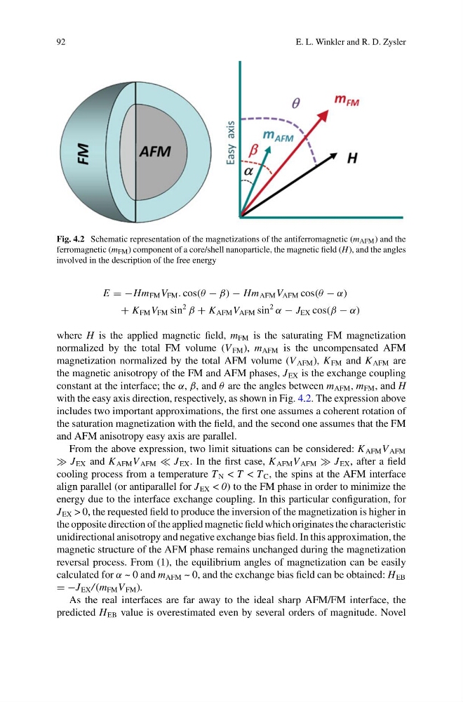
Fig. 4.2 Schematic representation of the magnetizations of the antiferromagnetic (m AFM ) and the
ferromagnetic (m FM ) component of a core/shell nanoparticle, the magnetic field (H), and the angles
involved in the description of the free energy
E = −Hm FM V FM . cos(θ − β) − Hm AFM V AFM cos(θ − α)
+ K FM V FM sin
2
β + K AFM V AFM sin
2
α − J EX cos(β − α)
where H is the applied magnetic field, m FM is the saturating FM magnetization
normalized by the total FM volume (V FM ), m AFM is the uncompensated AFM
magnetization normalized by the total AFM volume (V AFM ), K FM and K AFM are
the magnetic anisotropy of the FM and AFM phases, J EX is the exchange coupling
constant at the interface; the α, β, and θ are the angles between m AFM , m FM , and H
with the easy axis direction, respectively, as shown in Fig. 4.2. The expression above
includes two important approximations, the first one assumes a coherent rotation of
the saturation magnetization with the field, and the second one assumes that the FM
and AFM anisotropy easy axis are parallel.
From the above expression, two limit situations can be considered: K AFM V AFM
J EX and K AFM V AFM J EX . In the first case, K AFM V AFM J EX , after a field
cooling process from a temperature T N < T < T C , the spins at the AFM interface
align parallel (or antiparallel for J EX < 0) to the FM phase in order to minimize the
energy due to the interface exchange coupling. In this particular configuration, for
J EX > 0, the requested field to produce the inversion of the magnetization is higher in
the opposite direction of the applied magnetic field which originates the characteristic
unidirectional anisotropy and negative exchange bias field. In this approximation, the
magnetic structure of the AFM phase remains unchanged during the magnetization
reversal process. From (1), the equilibrium angles of magnetization can be easily
calculated for α ~ 0 and m AFM ~ 0, and the exchange bias field can be obtained: H EB
= −J EX / (m FM V FM ).
As the real interfaces are far away to the ideal sharp AFM/FM interface, the
predicted H EB value is overestimated even by several orders of magnitude. Novel
E. L. Winkler and R. D. Zysler
Fig. 4.2 Schematic representation of the magnetizations of the antiferromagnetic (m AFM ) and the
ferromagnetic (m FM ) component of a core/shell nanoparticle, the magnetic field (H), and the angles
involved in the description of the free energy
E = −Hm FM V FM . cos(θ − β) − Hm AFM V AFM cos(θ − α)
+ K FM V FM sin
2
β + K AFM V AFM sin
2
α − J EX cos(β − α)
where H is the applied magnetic field, m FM is the saturating FM magnetization
normalized by the total FM volume (V FM ), m AFM is the uncompensated AFM
magnetization normalized by the total AFM volume (V AFM ), K FM and K AFM are
the magnetic anisotropy of the FM and AFM phases, J EX is the exchange coupling
constant at the interface; the α, β, and θ are the angles between m AFM , m FM , and H
with the easy axis direction, respectively, as shown in Fig. 4.2. The expression above
includes two important approximations, the first one assumes a coherent rotation of
the saturation magnetization with the field, and the second one assumes that the FM
and AFM anisotropy easy axis are parallel.
From the above expression, two limit situations can be considered: K AFM V AFM
J EX and K AFM V AFM J EX . In the first case, K AFM V AFM J EX , after a field
cooling process from a temperature T N < T < T C , the spins at the AFM interface
align parallel (or antiparallel for J EX < 0) to the FM phase in order to minimize the
energy due to the interface exchange coupling. In this particular configuration, for
J EX > 0, the requested field to produce the inversion of the magnetization is higher in
the opposite direction of the applied magnetic field which originates the characteristic
unidirectional anisotropy and negative exchange bias field. In this approximation, the
magnetic structure of the AFM phase remains unchanged during the magnetization
reversal process. From (1), the equilibrium angles of magnetization can be easily
calculated for α ~ 0 and m AFM ~ 0, and the exchange bias field can be obtained: H EB
= −J EX / (m FM V FM ).
As the real interfaces are far away to the ideal sharp AFM/FM interface, the
predicted H EB value is overestimated even by several orders of magnitude. Novel