

76
C. H. Pyeon
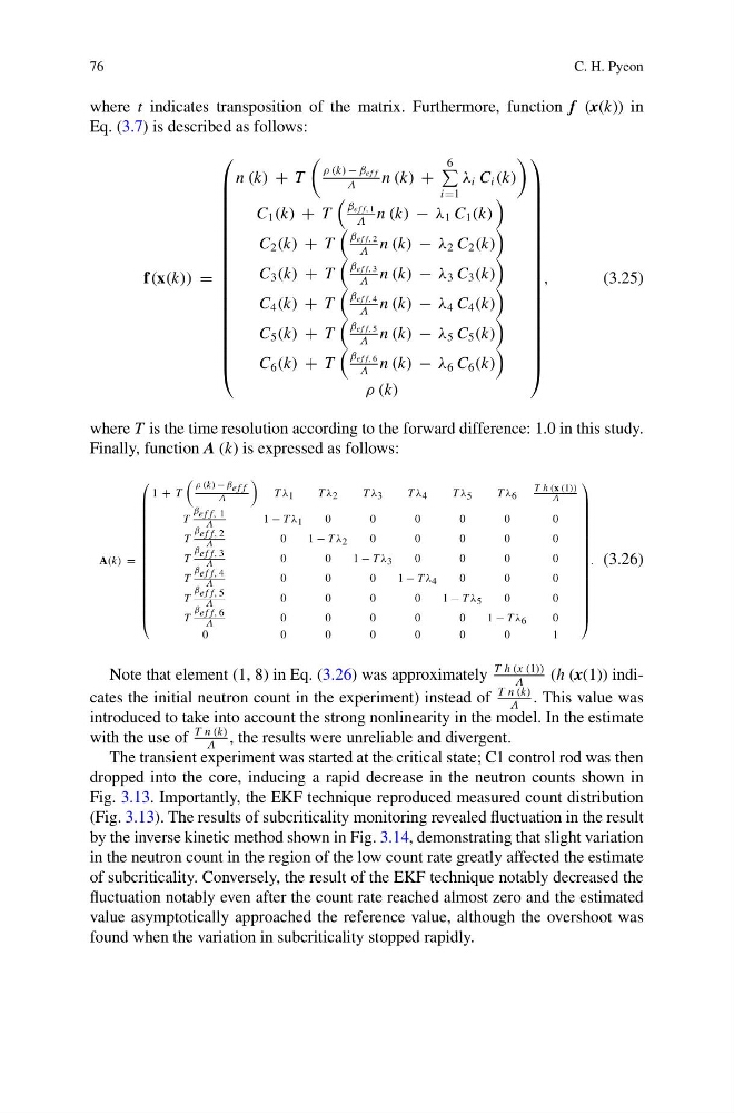
where t indicates transposition of the matrix. Furthermore, function f (x(k)) in
Eq. (3.7) is described as follows:
f(x(k)) =
⎛
⎜
⎜
⎜
⎜
⎜
⎜
⎜
⎜
⎜
⎜
⎜
⎜
⎜
⎜
⎜
⎜
⎜
⎜
⎝
n (k) + T
ρ (k) − β ef f
Λ
n (k) +
6
i=1
λ i C i (k)
C 1 (k) + T
β ef f, 1
Λ
n (k) − λ 1 C 1 (k)
C 2 (k) + T
β ef f, 2
Λ
n (k) − λ 2 C 2 (k)
C 3 (k) + T
β ef f, 3
Λ
n (k) − λ 3 C 3 (k)
C 4 (k) + T
β ef f, 4
Λ
n (k) − λ 4 C 4 (k)
C 5 (k) + T
β ef f, 5
Λ
n (k) − λ 5 C 5 (k)
C 6 (k) + T
β ef f, 6
Λ
n (k) − λ 6 C 6 (k)
ρ (k)
⎞
⎟
⎟
⎟
⎟
⎟
⎟
⎟
⎟
⎟
⎟
⎟
⎟
⎟
⎟
⎟
⎟
⎟
⎟
⎠
,
(3.25)
where T is the time resolution according to the forward difference: 1.0 in this study.
Finally, function A (k) is expressed as follows:
A(k) =
⎛
⎜
⎜
⎜
⎜
⎜
⎜
⎜
⎜
⎜
⎜
⎜
⎜
⎜
⎜
⎜
⎜
⎜
⎝
1 + T
ρ (k) − β ef f
Λ
T λ 1
T λ 2
T λ 3
T λ 4
T λ 5
T λ 6
T h (x (1))
Λ
T
β ef f, 1
Λ
1 − T λ 1
0
0
0
0
0
0
T
β ef f, 2
Λ
0
1− T λ 2
0
0
0
0
0
T
β ef f, 3
Λ
0
0
1− T λ 3
0
0
0
0
T
β ef f, 4
Λ
0
0
0
1− T λ 4
0
0
0
T
β ef f, 5
Λ
0
0
0
0
1− T λ 5
0
0
T
β ef f, 6
Λ
0
0
0
0
0
1− T λ 6
0
0
0
0
0
0
0
0
1
⎞
⎟
⎟
⎟
⎟
⎟
⎟
⎟
⎟
⎟
⎟
⎟
⎟
⎟
⎟
⎟
⎟
⎟
⎠
. (3.26)
Note that element (1, 8) in Eq. (3.26) was approximately
T h (x (1))
Λ
(h (x(1)) indicates the initial neutron count in the experiment) instead of
T n (k)
Λ
. This value was
introduced to take into account the strong nonlinearity in the model. In the estimate
with the use of
T n (k)
Λ
, the results were unreliable and divergent.
The transient experiment was started at the critical state; C1 control rod was then
dropped into the core, inducing a rapid decrease in the neutron counts shown in
Fig. 3.13. Importantly, the EKF technique reproduced measured count distribution
(Fig. 3.13). The results of subcriticality monitoring revealed fluctuation in the result
by the inverse kinetic method shown in Fig. 3.14, demonstrating that slight variation
in the neutron count in the region of the low count rate greatly affected the estimate
of subcriticality. Conversely, the result of the EKF technique notably decreased the
fluctuation notably even after the count rate reached almost zero and the estimated
value asymptotically approached the reference value, although the overshoot was
found when the variation in subcriticality stopped rapidly.
C. H. Pyeon
where t indicates transposition of the matrix. Furthermore, function f (x(k)) in
Eq. (3.7) is described as follows:
f(x(k)) =
⎛
⎜
⎜
⎜
⎜
⎜
⎜
⎜
⎜
⎜
⎜
⎜
⎜
⎜
⎜
⎜
⎜
⎜
⎜
⎝
n (k) + T
ρ (k) − β ef f
Λ
n (k) +
6
i=1
λ i C i (k)
C 1 (k) + T
β ef f, 1
Λ
n (k) − λ 1 C 1 (k)
C 2 (k) + T
β ef f, 2
Λ
n (k) − λ 2 C 2 (k)
C 3 (k) + T
β ef f, 3
Λ
n (k) − λ 3 C 3 (k)
C 4 (k) + T
β ef f, 4
Λ
n (k) − λ 4 C 4 (k)
C 5 (k) + T
β ef f, 5
Λ
n (k) − λ 5 C 5 (k)
C 6 (k) + T
β ef f, 6
Λ
n (k) − λ 6 C 6 (k)
ρ (k)
⎞
⎟
⎟
⎟
⎟
⎟
⎟
⎟
⎟
⎟
⎟
⎟
⎟
⎟
⎟
⎟
⎟
⎟
⎟
⎠
,
(3.25)
where T is the time resolution according to the forward difference: 1.0 in this study.
Finally, function A (k) is expressed as follows:
A(k) =
⎛
⎜
⎜
⎜
⎜
⎜
⎜
⎜
⎜
⎜
⎜
⎜
⎜
⎜
⎜
⎜
⎜
⎜
⎝
1 + T
ρ (k) − β ef f
Λ
T λ 1
T λ 2
T λ 3
T λ 4
T λ 5
T λ 6
T h (x (1))
Λ
T
β ef f, 1
Λ
1 − T λ 1
0
0
0
0
0
0
T
β ef f, 2
Λ
0
1− T λ 2
0
0
0
0
0
T
β ef f, 3
Λ
0
0
1− T λ 3
0
0
0
0
T
β ef f, 4
Λ
0
0
0
1− T λ 4
0
0
0
T
β ef f, 5
Λ
0
0
0
0
1− T λ 5
0
0
T
β ef f, 6
Λ
0
0
0
0
0
1− T λ 6
0
0
0
0
0
0
0
0
1
⎞
⎟
⎟
⎟
⎟
⎟
⎟
⎟
⎟
⎟
⎟
⎟
⎟
⎟
⎟
⎟
⎟
⎟
⎠
. (3.26)
Note that element (1, 8) in Eq. (3.26) was approximately
T h (x (1))
Λ
(h (x(1)) indicates the initial neutron count in the experiment) instead of
T n (k)
Λ
. This value was
introduced to take into account the strong nonlinearity in the model. In the estimate
with the use of
T n (k)
Λ
, the results were unreliable and divergent.
The transient experiment was started at the critical state; C1 control rod was then
dropped into the core, inducing a rapid decrease in the neutron counts shown in
Fig. 3.13. Importantly, the EKF technique reproduced measured count distribution
(Fig. 3.13). The results of subcriticality monitoring revealed fluctuation in the result
by the inverse kinetic method shown in Fig. 3.14, demonstrating that slight variation
in the neutron count in the region of the low count rate greatly affected the estimate
of subcriticality. Conversely, the result of the EKF technique notably decreased the
fluctuation notably even after the count rate reached almost zero and the estimated
value asymptotically approached the reference value, although the overshoot was
found when the variation in subcriticality stopped rapidly.