

72
C. H. Pyeon
x(k + 1) = f(x(k)) + bv(k),
(3.7)
y(k) = h(x(k)) + w(k),
(3.8)
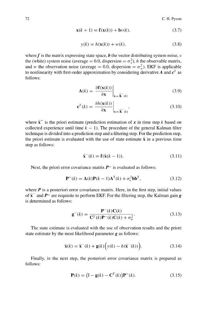
where f is the matrix expressing state space, b the vector distributing system noise, v
the (white) system noise (average = 0.0, dispersion = σ
2
v ), h the observable matrix,
and w the observation noise (average = 0.0, dispersion = σ
2
w ). EKF is applicable
to nonlinearity with first-order approximation by considering derivative A and c
T as
follows:
A(k) =
∂f(x(k))
∂x
x = x
− (k)
(3.9)
c
T
(k) =
∂h(x(k))
∂x
x = x
− (k)
,
(3.10)
where x
− is the priori estimate (prediction estimation of x in time step k based on
collected experience until time k − 1). The procedure of the general Kalman filter
technique is divided into a prediction step and a filtering step. For the prediction step,
the priori estimate is evaluated with the use of state estimate x
in a previous time
step as follows:
x
− (k) = f(x
(k − 1)).
(3.11)
Next, the priori error covariance matrix P − is evaluated as follows:
P
−
(k) = A(k)P(k − 1)A
T
(k) + σ
2
v bb
T
,
(3.12)
where P is a posteriori error covariance matrix. Here, in the first step, initial values
of x
− and P − are requisite to perform EKF. For the filtering step, the Kalman gain g
is determined as follows:
g
−
(k) =
P
−
(k)C(k)
C T (k)P − (k)C(k) + σ 2
w
.
(3.13)
The state estimate is evaluated with the use of observation results and the priori
state estimate by the most likelihood parameter g as follows:
x
(k) = x
− (k) + g(k)
y(k) − h(x
− (k))
.
(3.14)
Finally, in the next step, the posteriori error covariance matrix is prepared as
follows:
P(k) =
I − g(k) − C
T
(k)
P
−
(k).
(3.15)
C. H. Pyeon
x(k + 1) = f(x(k)) + bv(k),
(3.7)
y(k) = h(x(k)) + w(k),
(3.8)
where f is the matrix expressing state space, b the vector distributing system noise, v
the (white) system noise (average = 0.0, dispersion = σ
2
v ), h the observable matrix,
and w the observation noise (average = 0.0, dispersion = σ
2
w ). EKF is applicable
to nonlinearity with first-order approximation by considering derivative A and c
T as
follows:
A(k) =
∂f(x(k))
∂x
x = x
− (k)
(3.9)
c
T
(k) =
∂h(x(k))
∂x
x = x
− (k)
,
(3.10)
where x
− is the priori estimate (prediction estimation of x in time step k based on
collected experience until time k − 1). The procedure of the general Kalman filter
technique is divided into a prediction step and a filtering step. For the prediction step,
the priori estimate is evaluated with the use of state estimate x
in a previous time
step as follows:
x
− (k) = f(x
(k − 1)).
(3.11)
Next, the priori error covariance matrix P − is evaluated as follows:
P
−
(k) = A(k)P(k − 1)A
T
(k) + σ
2
v bb
T
,
(3.12)
where P is a posteriori error covariance matrix. Here, in the first step, initial values
of x
− and P − are requisite to perform EKF. For the filtering step, the Kalman gain g
is determined as follows:
g
−
(k) =
P
−
(k)C(k)
C T (k)P − (k)C(k) + σ 2
w
.
(3.13)
The state estimate is evaluated with the use of observation results and the priori
state estimate by the most likelihood parameter g as follows:
x
(k) = x
− (k) + g(k)
y(k) − h(x
− (k))
.
(3.14)
Finally, in the next step, the posteriori error covariance matrix is prepared as
follows:
P(k) =
I − g(k) − C
T
(k)
P
−
(k).
(3.15)