

3 Reactor Kinetics
71
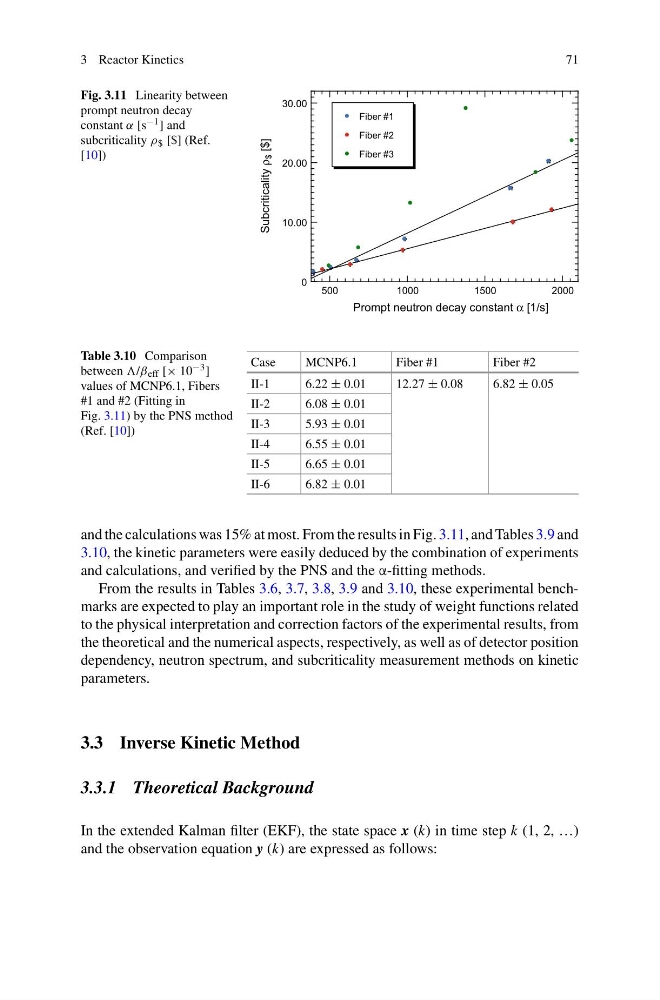
Fig. 3.11 Linearity between
prompt neutron decay
constant α [s −1 ] and
subcriticality ρ $ [$] (Ref.
[10])
500
1000
1500
2000
0
10.00
20.00
30.00
Prompt neutron decay constant α [1/s]
Subcriticality
ρ $ [$]
Fiber #1
Fiber #2
Fiber #3
Table 3.10 Comparison
between eff [× 10 −3 ]
values of MCNP6.1, Fibers
#1 and #2 (Fitting in
Fig. 3.11) by the PNS method
(Ref. [10])
Case
MCNP6.1
Fiber #1
Fiber #2
II-1
6.22 ± 0.01
12.27 ± 0.08
6.82 ± 0.05
II-2
6.08 ± 0.01
II-3
5.93 ± 0.01
II-4
6.55 ± 0.01
II-5
6.65 ± 0.01
II-6
6.82 ± 0.01
and the calculations was 15% at most. From the results in Fig. 3.11, and Tables 3.9 and
3.10, the kinetic parameters were easily deduced by the combination of experiments
and calculations, and verified by the PNS and the α-fitting methods.
From the results in Tables 3.6, 3.7, 3.8, 3.9 and 3.10, these experimental benchmarks are expected to play an important role in the study of weight functions related
to the physical interpretation and correction factors of the experimental results, from
the theoretical and the numerical aspects, respectively, as well as of detector position
dependency, neutron spectrum, and subcriticality measurement methods on kinetic
parameters.
3.3 Inverse Kinetic Method
3.3.1 Theoretical Background
In the extended Kalman filter (EKF), the state space x (k) in time step k (1, 2, …)
and the observation equation y (k) are expressed as follows:
71
Fig. 3.11 Linearity between
prompt neutron decay
constant α [s −1 ] and
subcriticality ρ $ [$] (Ref.
[10])
500
1000
1500
2000
0
10.00
20.00
30.00
Prompt neutron decay constant α [1/s]
Subcriticality
ρ $ [$]
Fiber #1
Fiber #2
Fiber #3
Table 3.10 Comparison
between eff [× 10 −3 ]
values of MCNP6.1, Fibers
#1 and #2 (Fitting in
Fig. 3.11) by the PNS method
(Ref. [10])
Case
MCNP6.1
Fiber #1
Fiber #2
II-1
6.22 ± 0.01
12.27 ± 0.08
6.82 ± 0.05
II-2
6.08 ± 0.01
II-3
5.93 ± 0.01
II-4
6.55 ± 0.01
II-5
6.65 ± 0.01
II-6
6.82 ± 0.01
and the calculations was 15% at most. From the results in Fig. 3.11, and Tables 3.9 and
3.10, the kinetic parameters were easily deduced by the combination of experiments
and calculations, and verified by the PNS and the α-fitting methods.
From the results in Tables 3.6, 3.7, 3.8, 3.9 and 3.10, these experimental benchmarks are expected to play an important role in the study of weight functions related
to the physical interpretation and correction factors of the experimental results, from
the theoretical and the numerical aspects, respectively, as well as of detector position
dependency, neutron spectrum, and subcriticality measurement methods on kinetic
parameters.
3.3 Inverse Kinetic Method
3.3.1 Theoretical Background
In the extended Kalman filter (EKF), the state space x (k) in time step k (1, 2, …)
and the observation equation y (k) are expressed as follows: