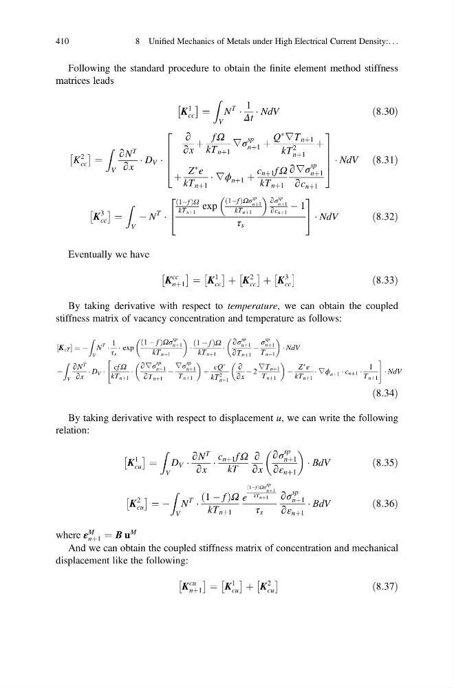
Following the standard procedure to obtain the finite element method stiffness
matrices leads
K
1
cc
 à ¼
Z
V
N
T
Á
1
Δt
Á NdV
ð8:30Þ
K
2
cc
 à ¼
Z
V
∂N
T
∂x
Á D V Á
∂
∂x
þ
f Ω
kT nþ1
∇σ
sp
nþ1 þ
Q
Ã
∇T nþ1
kT
2
nþ1
þ
þ
Z
à e
kT nþ1
Á ∇ϕ nþ1 þ
c nþ1 f Ω
kT nþ1
∂∇σ
sp
nþ1
∂c nþ1
2
6
6
6
4
3
7
7
7
5
Á NdV ð8:31Þ
K
3
cc
 à ¼
Z
V
À N
T
Á
1Àf
ð
ÞΩ
kT nþ1
exp
1Àf
ð
ÞΩσ
sp
nþ1
kT nþ1
∂σ
sp
nþ1
∂c nþ1
À 1
τ s
2
4
3
5 Á NdV
ð8:32Þ
Eventually we have
K
cc
nþ1
Â
à ¼ K
1
cc
 à þ K
2
cc
 à þ K
3
cc
 Ã
ð8:33Þ
By taking derivative with respect to temperature, we can obtain the coupled
stiffness matrix of vacancy concentration and temperature as follows:
K cT
½
Š¼À
Z
V
N
T Á
1
τ s
Á exp
1 À f
ð
ÞΩσ
sp
nþ1
kT nþ1
Á
1 À f
ð
ÞΩ
kT nþ1
Á
∂σ
sp
nþ1
∂T nþ1
À
σ
sp
nþ1
T nþ1
Á NdV
þ
Z
V
∂N
T
∂x
Á D V Á
cf Ω
kT nþ1
Á
∂∇σ
sp
nþ1
∂T nþ1
À
∇σ
sp
nþ1
T nþ1
þ
cQ
Ã
kT
2
nþ1
∂
∂x
À 2
∇T nþ1
T nþ1
À
Z
à e
kT nþ1
Á ∇ϕ nþ1 Á c nþ1 Á
1
T nþ1
"
#
Á NdV
ð8:34Þ
By taking derivative with respect to displacement u, we can write the following
relation:
K
1
cu
 à ¼
Z
V
D V Á
∂N
T
∂x
Á
c nþ1 f Ω
kT
∂
∂x
∂σ
sp
nþ1
∂ε nþ1
Á ΒdV
ð8:35Þ
K
2
cu
 à ¼ À
Z
V
N
T
Á
1 À f
ð
ÞΩ
kT nþ1
e
1Àf
ð
Þ Ωσ
sp
nþ1
kT nþ1
τ s
∂σ
sp
nþ1
∂ε nþ1
Á ΒdV
ð8:36Þ
where ε
M
nþ1 ¼ Β u
M
And we can obtain the coupled stiffness matrix of concentration and mechanical
displacement like the following:
K
cu
nþ1
Â
à ¼ K
1
cu
 à þ K
2
cu
 Ã
ð8:37Þ
410
8 Unified Mechanics of Metals under High Electrical Current Density:. . .