

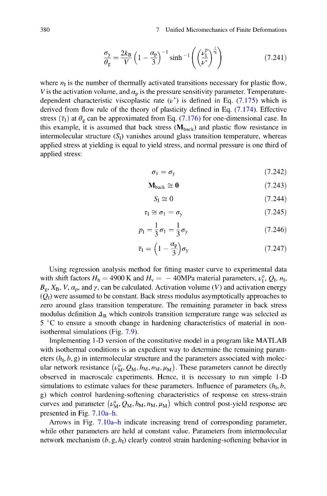
σ y
θ g
¼
2k B
V
1 À
α p
3
À1
sinh
À1
ν
p
I
ν Ã
1
n I
!
ð7:241Þ
where n I is the number of thermally activated transitions necessary for plastic flow,
V is the activation volume, and α p is the pressure sensitivity parameter. Temperaturedependent characteristic viscoplastic rate (ν
à ) is defined in Eq. (7.175) which is
derived from flow rule of the theory of plasticity defined in Eq. (7.174). Effective
stress τ I
ð Þ at θ g can be approximated from Eq. (7.176) for one-dimensional case. In
this example, it is assumed that back stress (M back ) and plastic flow resistance in
intermolecular structure (S I ) vanishes around glass transition temperature, whereas
applied stress at yielding is equal to yield stress, and normal pressure is one third of
applied stress:
σ 1 ¼ σ y
ð7:242Þ
M back ffi 0
ð7:243Þ
S I ffi 0
ð7:244Þ
τ I ffi σ 1 ¼ σ y
ð7:245Þ
p I ¼
1
3
σ 1 ¼
1
3
σ y
ð7:246Þ
τ I ¼ 1 À
α p
3
σ y
ð7:247Þ
Using regression analysis method for fitting master curve to experimental data
with shift factors H h ¼ 4900 K and H v ¼ À 40MPa material parameters, ν
o
I , Q I , n I ,
B g , X B , V, α p , and γ, can be calculated. Activation volume (V ) and activation energy
(Q I ) were assumed to be constant. Back stress modulus asymptotically approaches to
zero around glass transition temperature. The remaining parameter in back stress
modulus definition Δ B which controls transition temperature range was selected as
5
C to ensure a smooth change in hardening characteristics of material in nonisothermal simulations (Fig. 7.9).
Implementing 1-D version of the constitutive model in a program like MATLAB
with isothermal conditions is an expedient way to determine the remaining parameters (h I , b, g) in intermolecular structure and the parameters associated with molecular network resistance ν
o
M , Q M , h M , n M , μ M
À
Á
. These parameters cannot be directly
observed in macroscale experiments. Hence, it is necessary to run simple 1-D
simulations to estimate values for these parameters. Influence of parameters (h I , b,
g) which control hardening-softening characteristics of response on stress-strain
curves and parameter ν
o
M , Q M , h M , n M , μ M
À
Á
which control post-yield response are
presented in Fig. 7.10a–h.
Arrows in Fig. 7.10a–h indicate increasing trend of corresponding parameter,
while other parameters are held at constant value. Parameters from intermolecular
network mechanism (b, g, h I ) clearly control strain hardening-softening behavior in
380
7 Unified Micromechanics of Finite Deformations
θ g
¼
2k B
V
1 À
α p
3
À1
sinh
À1
ν
p
I
ν Ã
1
n I
!
ð7:241Þ
where n I is the number of thermally activated transitions necessary for plastic flow,
V is the activation volume, and α p is the pressure sensitivity parameter. Temperaturedependent characteristic viscoplastic rate (ν
à ) is defined in Eq. (7.175) which is
derived from flow rule of the theory of plasticity defined in Eq. (7.174). Effective
stress τ I
ð Þ at θ g can be approximated from Eq. (7.176) for one-dimensional case. In
this example, it is assumed that back stress (M back ) and plastic flow resistance in
intermolecular structure (S I ) vanishes around glass transition temperature, whereas
applied stress at yielding is equal to yield stress, and normal pressure is one third of
applied stress:
σ 1 ¼ σ y
ð7:242Þ
M back ffi 0
ð7:243Þ
S I ffi 0
ð7:244Þ
τ I ffi σ 1 ¼ σ y
ð7:245Þ
p I ¼
1
3
σ 1 ¼
1
3
σ y
ð7:246Þ
τ I ¼ 1 À
α p
3
σ y
ð7:247Þ
Using regression analysis method for fitting master curve to experimental data
with shift factors H h ¼ 4900 K and H v ¼ À 40MPa material parameters, ν
o
I , Q I , n I ,
B g , X B , V, α p , and γ, can be calculated. Activation volume (V ) and activation energy
(Q I ) were assumed to be constant. Back stress modulus asymptotically approaches to
zero around glass transition temperature. The remaining parameter in back stress
modulus definition Δ B which controls transition temperature range was selected as
5
C to ensure a smooth change in hardening characteristics of material in nonisothermal simulations (Fig. 7.9).
Implementing 1-D version of the constitutive model in a program like MATLAB
with isothermal conditions is an expedient way to determine the remaining parameters (h I , b, g) in intermolecular structure and the parameters associated with molecular network resistance ν
o
M , Q M , h M , n M , μ M
À
Á
. These parameters cannot be directly
observed in macroscale experiments. Hence, it is necessary to run simple 1-D
simulations to estimate values for these parameters. Influence of parameters (h I , b,
g) which control hardening-softening characteristics of response on stress-strain
curves and parameter ν
o
M , Q M , h M , n M , μ M
À
Á
which control post-yield response are
presented in Fig. 7.10a–h.
Arrows in Fig. 7.10a–h indicate increasing trend of corresponding parameter,
while other parameters are held at constant value. Parameters from intermolecular
network mechanism (b, g, h I ) clearly control strain hardening-softening behavior in
380
7 Unified Micromechanics of Finite Deformations